
Confidence intervals 2/3: bootstrapping methods
Learn computational statistics in the second part of this three-part series.

About this three-part series
Welcome to the second part of the series! The previous post was an introduction to confidence intervals and the analytic formula to calculate them. This second post is focused on empirical methods to get confidence intervals without making assumptions on your data characteristics or distributions.
I use code to help teach data science, because you can learn a lot of math with a bit of code. The essential code bits are shown in this post, and the full code files are on my GitHub page. I encourage you to run the code as you’re reading this post.
When to use empirical (a.k.a. computational, a.k.a. non-parametric) confidence intervals?
In the previous post, you learned two limitations of analytic confidence intervals (CI):
The analytic method depends on assumptions on the data.
The analytic method is defined only for certain statistical parameters (e.g., sample average or regression coefficient), whereas many other statistical characteristics do not have a known analytic CI formula.
These limitations motivate the use of empirical CIs, which are also called computational or non-parametric CIs. The primary method of obtaining empirical CIs is bootstrapping, and the primary application is determining whether a finding is statistically significant.
In this post, I will explain what bootstrapping means and why it works, then show a code demo of bootstrap CIs in simulated data. In part 3 of this post series, I will show two applications of confidence intervals in a real dataset.
What is bootstrapping and how does it work?
“Bootstrapping” is an algorithm in computational statistics that involves calculating a sample characteristic (such as an average, median, standard deviation, correlation coefficient, etc.) from the same dataset, sampling randomly and with replacement.
That’s a mouthful. Let me explain using a simple example.
Consider the dataset [1,2,3,4]. The average of that dataset is 2.5. Now let’s draw a random sample from that dataset with sample size = 4:
[2,1,1,4] → average = 2.
Huh, so the number “1” was sampled twice while the number “3” wasn’t sampled at all. That happens when you randomly sample with replacement. Each time you pick a number from the dataset, you put that number back in so it could be sampled more than once. That also means that the average can be different from the original average.
In other words, there is uncertainty associated with the sample average that the random resampling reveals. That’s not an artifact — it is intrinsic to the dataset but you can’t see it just by looking at the data; you need to resample to observe that variability. As a counter-example, imagine a dataset [2,2,2,2]. It doesn’t matter how often you resample, the average will always be 2.
I resampled the data five times and calculated the average; the resamples and their averages are below (the first row is the original data).
    Sample    |  Mean
----------------------
[1, 2, 3, 4]  |  2.50
[1, 1, 3, 4]  |  2.25
[1, 3, 3, 4]  |  2.75
[2, 2, 3, 4]  |  2.75
[1, 1, 2, 2]  |  1.50
[2, 2, 2, 4]  |  2.50
In theory, the average could be as low as 1 or as high as 4, although in practice, we’d expect most of the resampled averages to be closer to 2.5.
And that’s the basics of random resampling.
Calculating CIs via bootstrapping
Bootstrapping involves resampling hundreds or thousands of times to get a distribution of data characteristics, and then finding the values at 2.5% and 97.5% of that distribution.
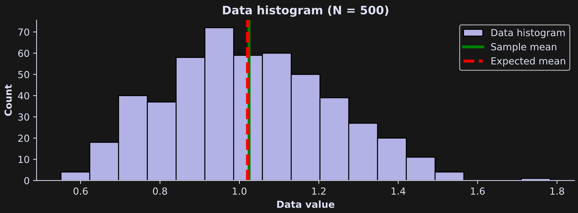
Let’s work through a demo. I will generate random numbers from a lognormal distribution with a known population mean. (A lognormal distribution is defined as exp(x) where x is normally distributed numbers.)
Figure 1 below shows a histogram of the data, the theoretical expected average (dashed red line) and the sample average (green line).
Our goal now will be to get the 95% confidence interval of the sample average, and then compare that to the expected value. Here’s the code to get one resampled average.
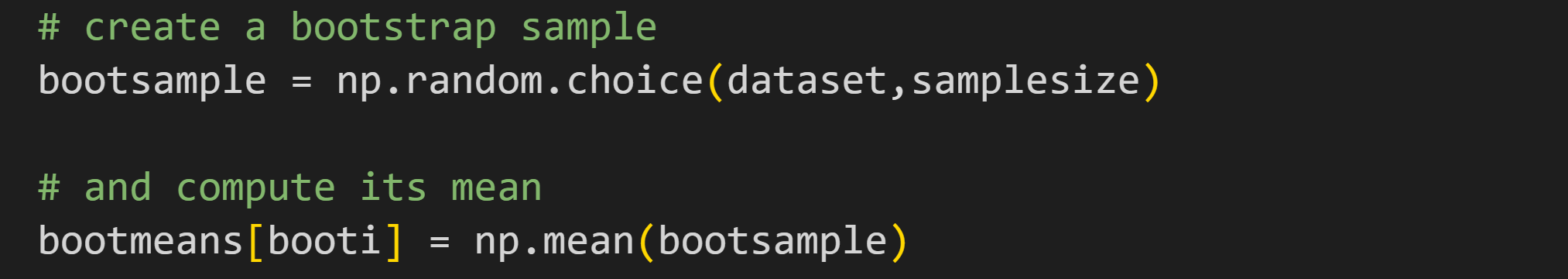
The choice() function in numpy’s random module selects samplesize (500 in this demo) samples randomly from the numbers in variable dataset. By default, this function has replacement=True, which means the same data values could be drawn repeatedly, while others could be left out.
That code is put inside a for-loop over 1000 iterations (variable booti is the looping index). After that for-loop, we have 1000 reshuffled means in variable bootmeans. That’s the bootstrapping.
I visualized the results in Figure 2 below. There’s a lot going on in those plots! I will provide explanations below the figure, but before reading further, I want you to spend a moment looking at the figure and see what you understand, what conclusions you can draw, and what questions you have.
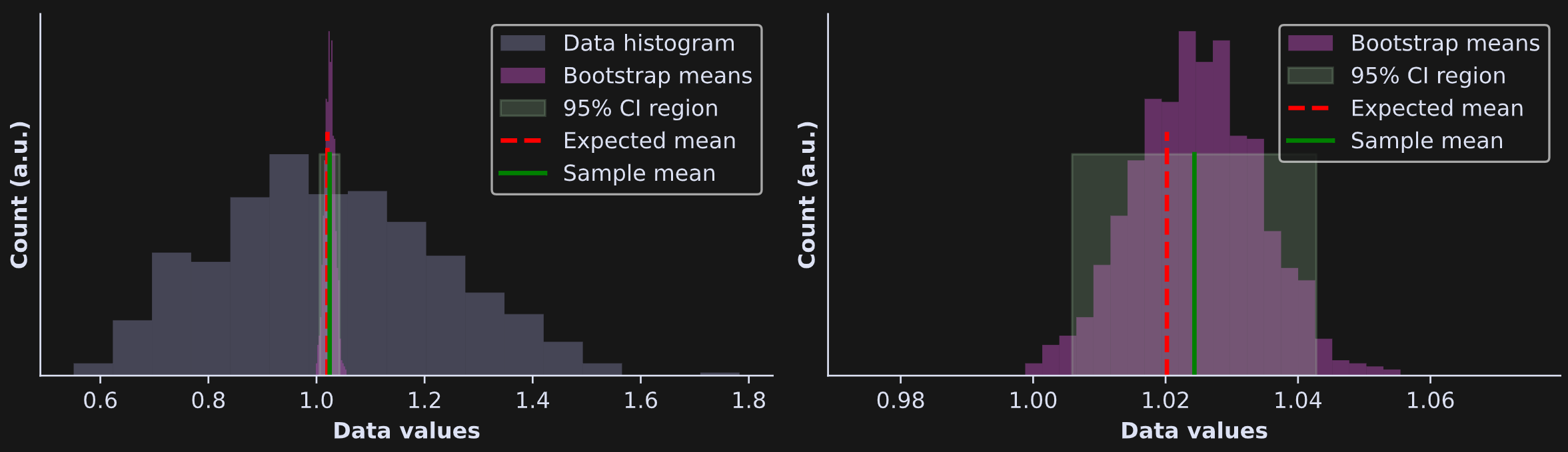
The left panel shows the same histogram as in Figure 1, but with a light green box drawn on top indicating the 95% CI bounds. To be honest, it’s really difficult to see that green box, because the CIs are so narrow. That’s why I zoomed-in to the plot in the right-side panel (note the x-axis values in the two plots).
The light pink histogram is not of the data; it’s of the resampled averages. The distribution of bootstrapped averages will be tighter than the histogram of the data. (And fun fact: That bootstrapped distribution will always look Gaussian, even when the data are non-normally distributed, thanks to the Central Limit Theorem.)
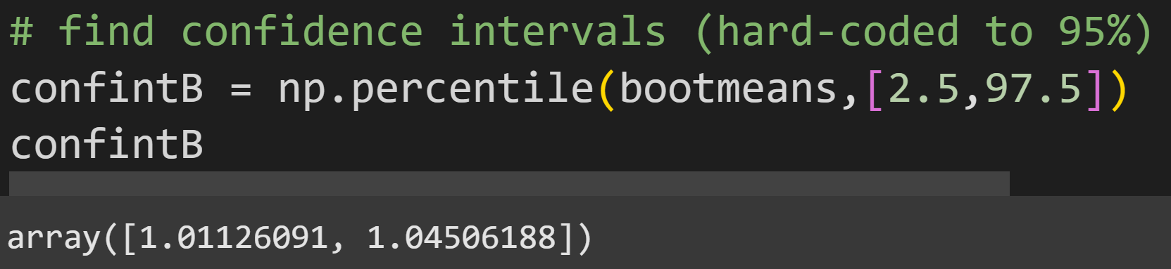
The green rectangle shows the 95% CI around the sample mean (the green line). How did I calculate the CI? I used numpy’s percentile function to get the 2.5% and 97.5% of the distribution. In other words, 95% of the bootstrap means were in between 1.011 and 1.045.
Back to Figure 2: The red line (expected population average) is inside the 95% CI boundaries. What does that mean? It means that the true population mean was within the CI bounds of the sample, which we can interpret as indicating that the sample was drawn from a population with that average. In other words, the sample average is numerically different from the population average, but it’s not statistically significantly different from the population average. Of course, that’s not surprising: I generated the data from that distribution. In Part 3 of this series, you’ll get to explore bootstrap statistical significance in real data.
Bootstrap CIs for other statistical characteristics
Any characteristic you can calculate, you can get CIs on. The figure below shows the same CI procedure as above, using the same dataset, but for the standard deviation instead of the average.
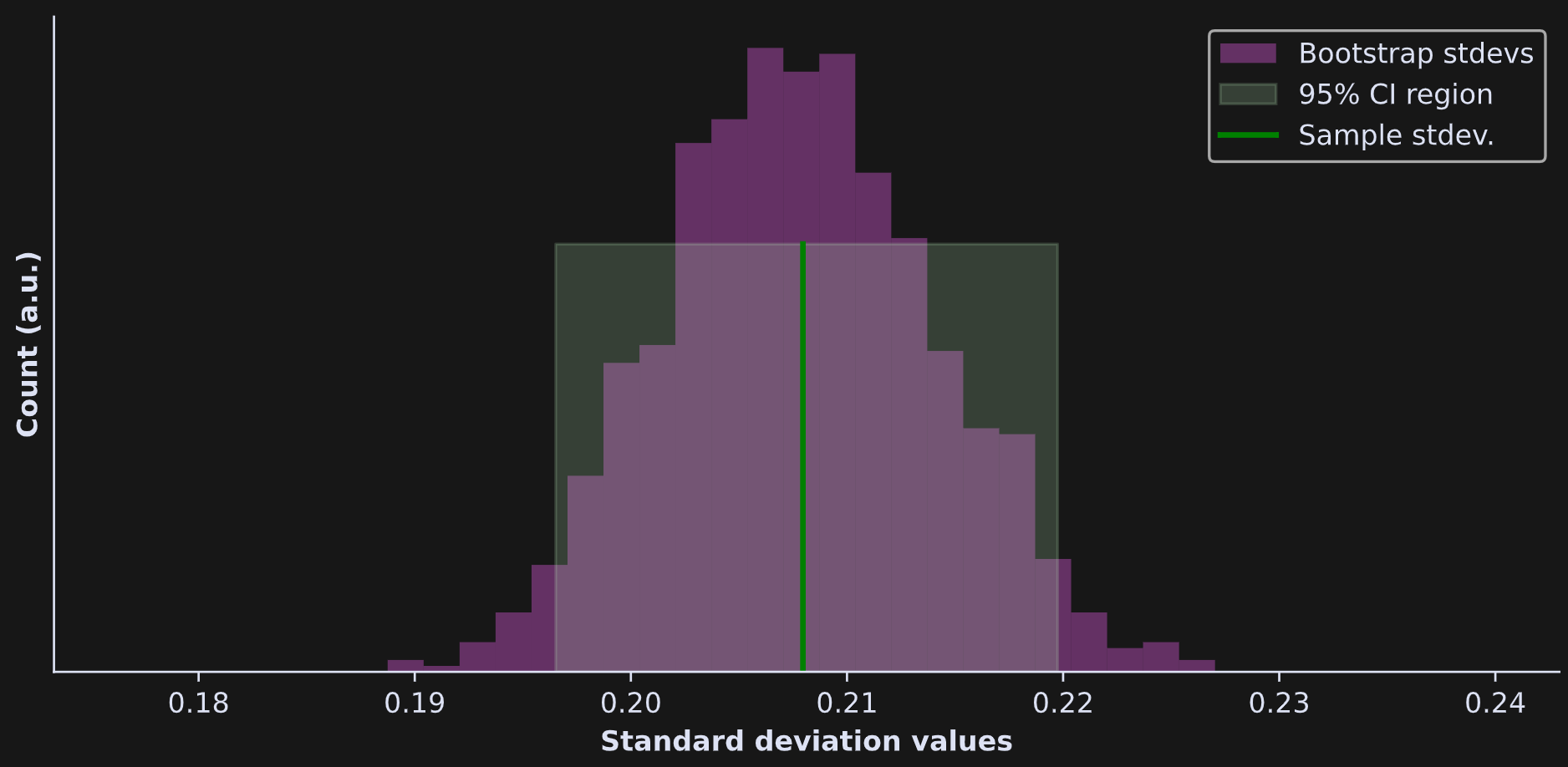
In fairness, there are analytic methods to get the CI of a sample standard deviation, but this example highlights the versatility of empirical CIs: All you need to do is resample and recompute, and you can get CIs. That is particularly relevant for modern machine-learning methods, for which analytic CIs may not exist or assumptions like normality are violated.
Common questions about bootstrapping
How are the bootstrap and analytic CIs related?
If the data are normally distributed, there are no outliers or other extreme values, and the sample size is “reasonable” (e.g., >30), then the bootstrap and analytic CIs will be very close.
I calculated the CIs using both methods in the dataset shown above. You can see in the results below that the range is quite comparable. (Formally, the data are lognormal, not normal, but the distribution is close enough to normal that the analytic formula is valid.)
Empirical CI(95%) = (1.011,1.045)
Analytic  CI(95%) = (1.008,1.049)
On the other hand, if the data are non-normally distributed or have outliers or non-representative values, then the analytic and bootstrap approaches can give very different results. In these cases, you could either clean the data or prefer the computational over the analytic approach.
How many resamples?
The secret is this: you don’t care about the resampled distribution. Instead, you care about the percentiles of that distribution. So question is really this: How many resamples do you need to get an accurate estimate of the 2.5/97.5 percentiles? Obviously, you need more than one. But do you need 100? 1000? 1 bajillion?
There is no magic number of resamples to use. Most people resample hundreds or a few thousand times. If you have very clean data, you might only need 100, and if you have noisy data with a lot of variability or outliers, then you might need several thousand.
To explore this idea, I ran an experiment with the simulated data from earlier. I re-calculated CI widths in the same data, in a for-loop over 10 to 10,000 bootstrap samples. Those results are in Figure 4. CI width generally stabilized as the number of resamples increased, although there was still variability even going up to 10k samples.
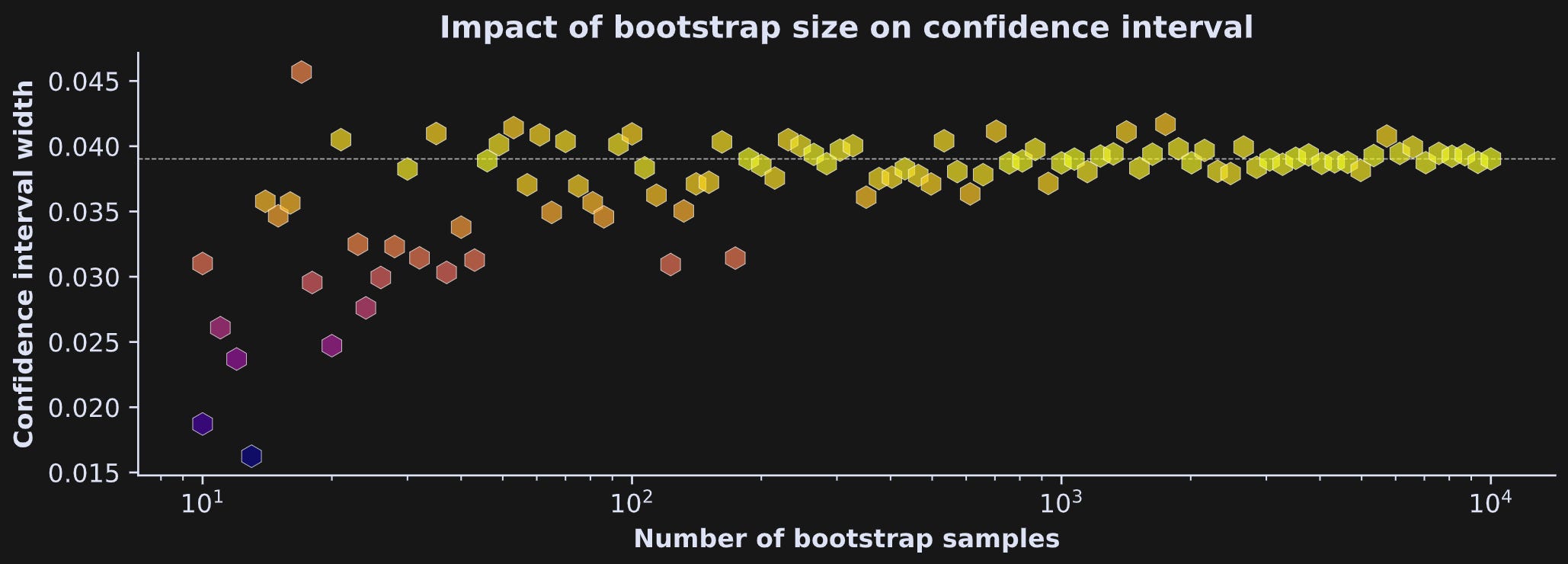
To be clear: Each individual bootstrap mean comes from resampling N times (that, is, the samplesize parameter of np.random.choice is always the same). Instead, what x-axis shows is the number of sample averages that I used to calculate the 95% confidence intervals.
This is just one simulation in one dataset, so don’t over-interpret this result. But this pattern of findings is quite consistent for bootstrapping: More resamples helps, but there is still variability in the CIs even with a large number of resamples.
There are also practical considerations. If you’re only running one analysis like in this post, then you can run 10,000,000 resamples and it might take a few seconds. But imagine you have multiple huge datasets and need to calculate CIs for hundreds or thousands of parameters. Furthermore, some analyses are computationally simple (e.g., averaging numbers) while other analyses are computationally expensive (e.g., a spectral analysis on time series data). If each resample takes 1 second, and you do 100,000 resamples, and you have 400 datasets to process, then, well, I hope your boss is very patient and your project isn’t urgent.
Why does the resample have the same sample size?
In the examples I showed in this post, the resample size was the same as the original sample size. Why not take smaller or larger samples?
The most important reason is that the resampled dataset should have comparable characteristics as the original dataset. Under-sampling or over-sampling risks the bootstrap distribution being too different from the original data.
Another reason is just for convenience of justification and avoiding unnecessary arbitrary choices. Let’s say you resample with N-2 samples. People would ask you to justify why you sampled N-2 — and why not N-1 or N-14. There are many arbitrary choices in statistics (p<.05 has entered the chat…), but at least if we all do it consistently, then we build convention and consensus.
Why is it called “bootstrapping” lol?
Have you heard the expression pull yourself up by your bootstraps? It’s an absurdity: Imagine trying to lift yourself off the ground by pulling up on your shoelaces. It’s literally impossible. Figuratively, that expression refers to doing something difficult by sheer willpower. For example, it would be a compliment to someone who grew up poor and uneducated, then became a successful self-taught engineer.
In the context of confidence intervals, we are doing the impossible: Estimating bounds for a population parameter without knowing the population parameter.
And that’s a good segue to the assumptions of empirical CIs.
Assumptions of empirical CIs
Some people think that computational and non-parametric statistics have no assumptions. That’s not true. It is true that the assumptions are fewer and “softer” (that is, less mathematically defined and rigorous) than parametric statistics and analytic CIs. Here are the assumptions of bootstrapped CIs:
The sample is representative of the population. If you want to generalize from your sample to a population then your sample has to be representative. As an extreme counter-example: If you want to know the average height of Montenegrin basketball players, you cannot sample heights of Belarussian children.
Of course, having samples that are random and independent is a good way to ensure that the sample is representative of the population.Large enough sample. Here again you see this nebulous advice to have a “big enough” sample. The ambiguity of appropriate sample size permeates nearly every discussion in applied statistics. In the context of bootstrap confidence intervals, the sample needs to be big enough to create a distribution from which the 2.5/97.5% values can be estimated. For example, the first demo of bootstrapping from this post had only four numbers; that’s enough to illustrate the mechanism but not enough to have a reliable statistical estimate.
What about other assumptions, like normality and equal variance? Those don’t matter! Violate those assumptions to your heart’s delight :)

Here’s the neat part: any “weird” characteristics in your data, including non-normal distributions, unequal variances, and outliers, get incorporated into the bootstrapped distribution.
All that said, it is best to have high-quality, clean data. All statistical procedures are GIGO boxes (garbage in, garbage out). Bootstrapped CIs are great, and they have several advantages over analytic CIs especially in modern machine-learning analyses; but they’re not magic bullets that can fix crappy data.
Increase my sample size :P
I write these posts because I want to bring high-quality technical education to as many people as possible — but also because it’s my job and my source of income. Please consider supporting me by enrolling in my online courses, buying my books, or becoming a paid subscriber here on Substack. If you have a tight budget, then please keep your money for more important things, and instead just share these links.