
DDC-23: Distributions of MNIST pixel values
A data challenge a day helps you master machine learning

About these daily data challenges
Each post is an exercise that helps you learn about data in Python.
Try to solve the exercise before checking my solution at the bottom of the post 🤓
You can share your solution or visualization in the comments!
Today’s challenge
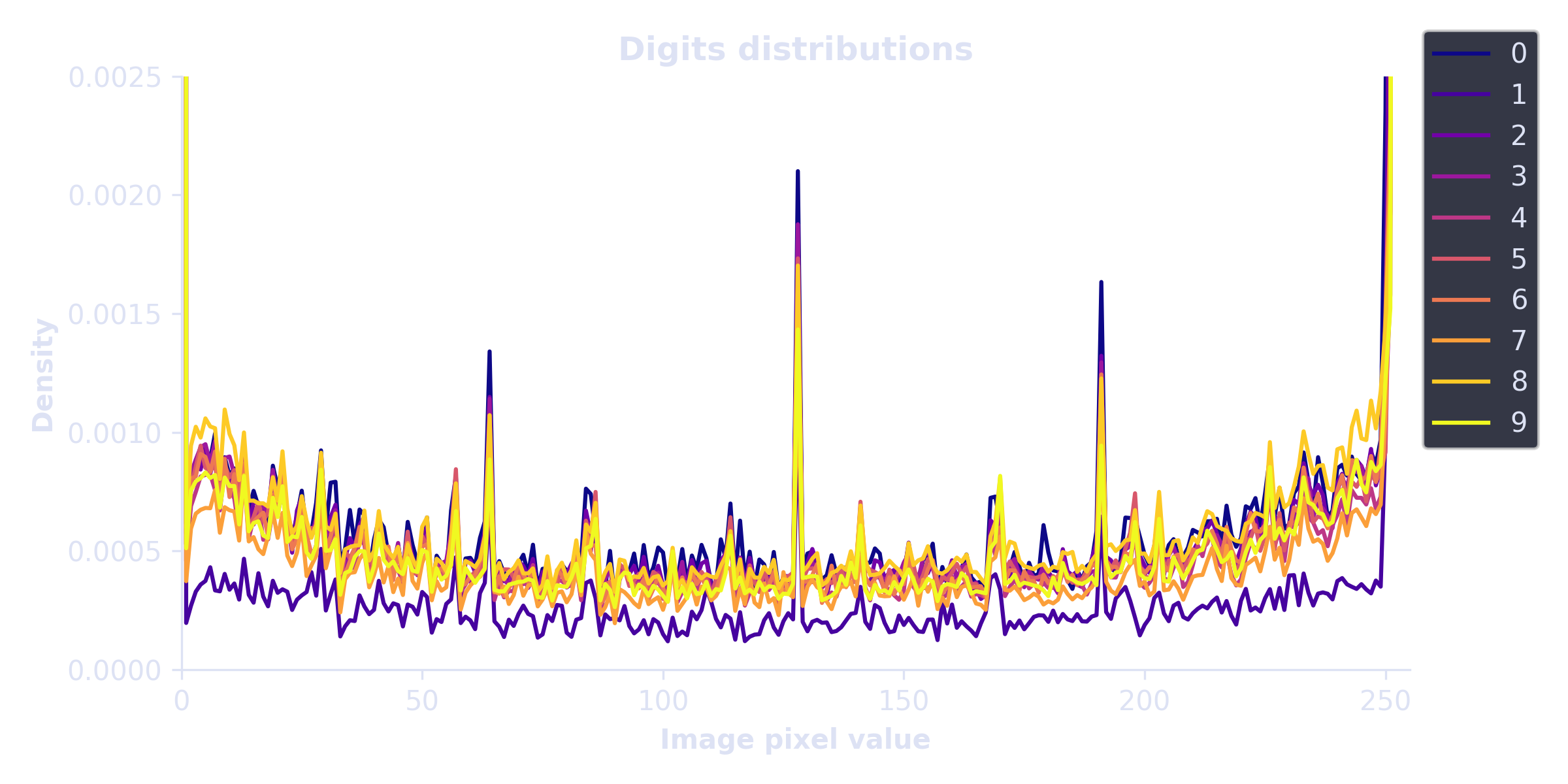
This is the same dataset as in the DDC-22. Your goal here is to visualize the distributions (histograms) of the image pixel intensities for each digit.
Data can be imported directly from Google Colab (filename mnist_train_small.csv). Import the data using the numpy library (do not use pandas for this DDC). The dataset is an array of 20,000 by 785, corresponding to 20k samples and 784 pixels that you need to reshape to a 28x28 matrix. The first column is the digit label.
Use np.histogram to get the density distribution of pixel values for all samples from each digit, using integer bin boundaries between 0 and 255. Draw each distribution as a separate line in the same plot, as below. Most of the pixels are either zero or 255, so you should adjust the y-axis limits to make the rest of the distribution visible.
.
.
.
.
Scroll down for the solution!
.
.
.
.

.
.
.
.
Keep scrolling!
.
.
.
.
import numpy as np
import matplotlib.pyplot as plt

# import data
mnist = np.loadtxt('/content/sample_data/mnist_train_small.csv', delimiter=',')

# histogram bin edges (using integers)
bins = np.arange(0,256)

plt.figure(figsize=(8,4))
for num in range(10):
  thisnum = mnist[mnist[:,0]==num,1:].flatten()
  y,x = np.histogram(thisnum,bins=bins,density=True)
  plt.plot(bins[:-1],y,color=mpl.cm.plasma(num/9),label=f'{num}')

plt.legend(bbox_to_anchor=[1,1.1])
plt.gca().set(xlabel='Image pixel value',ylabel='Density',title='Digits distributions',
              xlim=bins[[0,-1]],ylim=[0,.0025])
plt.tight_layout()
plt.show()