Effective dimensionality analysis of LLM transformers

How many dimensions does GPT need to process text and code?

Before you begin: You can follow along with Python to recreate the figures and demos, and modify the experiments, using the code file posted on my GitHub.

The video below shows how to start working with the code.

What is “effective dimensionality”?

Consider a flat sheet of paper. It is technically three-dimensional (let’s ignore for the moment fringe-string-theory proposals of a dozen additional curled-up spatial dimensions), but it has only two effective dimensions: height and width. The thickness of the paper is multiple orders of magnitude smaller than the other two dimensions, and you cannot use the thickness dimension in any practical way to convey information.

Thus, the paper is technically 3D but there are only two dimensions that can be used to store and convey information. So, the effective dimensionality is 2D.

Figure 1 shows another example with data. The left panel shows dots that all lie on a line in a 2D graph. Two dimensions but an effective dimensionality of 1.

The right panel is a little more interesting and ambiguous. The dots do not lie exactly on the line. What is the effective dimensionality of that dataset?

Figure 1: Left panel shows a dataset that is technically 2-dimensional but has only one dimension of information — a diagonal line. Right panel shows a dataset with an effective dimensionality of one or two, depending on your assumptions about the minor deviations.

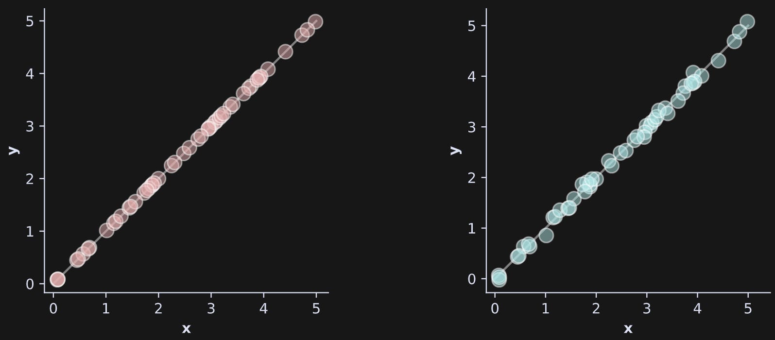
The answer is that it depends on assumptions we make. If we assume that the minor divergences off the line are pure noise — just tiny random errors that convey no information — then we can still consider the effective dimensionality to be 1. On the other hand, if we assume that the divergences are meaningful even though they are tiny, then we would consider the effective dimensionality to be 2.

In practical dimensionality analyses, we apply some threshold to the results. For example, we might say that a dimension in the data space needs to account for at least 1% of the total variability in the data to be counted. That’s analogous to saying that the thickness of a piece of paper is excluded from our dimensionality count because it accounts for less than 1% of the volume.

Measuring effective dimensionality with the SVD

The singular value decomposition (SVD) is a real gem of linear algebra, and because (imho) linear algebra is a real gem of mathematics, the SVD is one of the most elegant operations in applied math. It’s used in myriad applications, including principal components analysis (PCA), ML classifiers, image compression, signal processing, and computational sciences including physics, biology, engineering, and finance.

The goal of an SVD is to break apart a matrix into a trio of other matrices that reveal important yet hidden features of the matrix. Imagine breaking apart the number 101.01 into:

OK, I admit that for this example, the three smaller pieces don’t exactly reveal any hidden secrets in the number 101.01, but we have decomposed one number into three simpler pieces. And that’s the idea.

With matrices, the concept is similar but the hidden secrets in the matrix are much more hidden.

Figure 2: Graphical overview of the SVD. An embeddings matrix (left) is decomposed into the product of three matrices. For dimensionality analysis, we only need the Σ matrix that encodes the “importance” or “thickness” of each dimension.

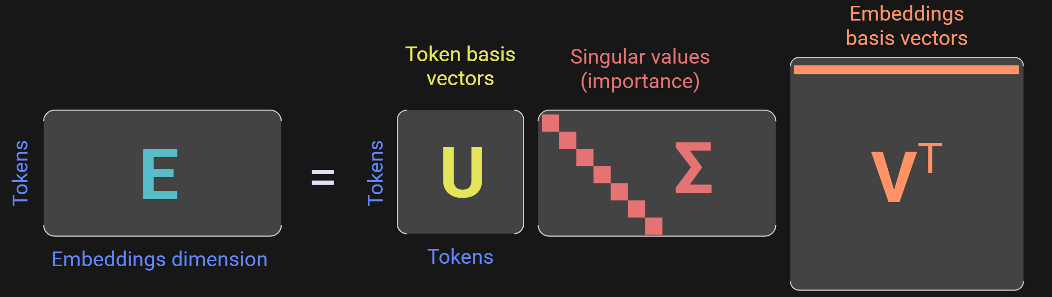
It would take more than a few short paragraphs without equations to explain the full SVD, but for the purposes of dimensionality analysis, you only need to know one part of the SVD, which is the singular values (middle matrix in Figure 2). The singular values encode the “importance” or the “thickness” of each dimension in the data space. The sum of all singular values is the total variability in the data.

To continue with the paper analogy, the SVD of a US-standard piece of paper would have singular values of [11, 8, .005] in units of inches. (Important to know: the singular values are sorted descending.)

Here’s how to interpret the singular value spectrum: A simple system has few “moving parts” and therefore most of its variance is captured by one or a small number of components. In contrast, a complex system has a lot of distinct moving parts and subsystems, and therefore its variance is distributed over multiple separate components. This is diagrammed in the figure below.

Figure 3: Conceptual overview of singular value spectra for a simple vs. a complex system.

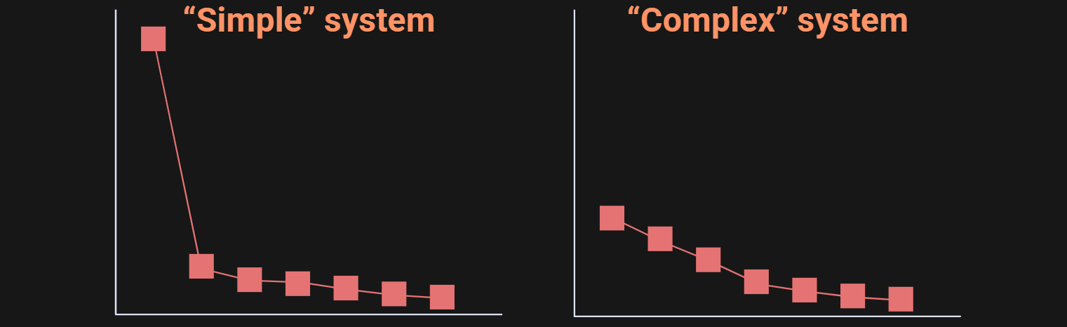
In the figure, I used the terms “simple” and “complex” in apology quotes, because an SVD alone should not be used to categorize systems as simple or complex. On the other hand, it is the case that complex systems with multiple dynamical and independent subsystems will have a singular value spectrum that decays more gradually.

Anyway, Figure 3 shows a qualitative interpretation. We need to quantify the shape of the distribution and then define our measure of “effective dimensionality.” And to do that, we need to transform the singular values.

The “raw” singular values are difficult to interpret on their own because their numerical scaling depends on the data — multiply the dataset by 2 and the singular values will increase, even though the patterns in the data are the same. That is to say, if I told you that one matrix has a largest singular value of 4.5 and another matrix has a largest singular value of 8.2, there is really nothing you can conclude about the two matrices: they could differ in scale or complexity (or both).

That’s why, for many applications include dimensionality analysis and principal components analysis, the singular values are often transformed to percent total variance.

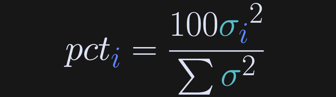
pct is the percentage of total variance explained by the i-th component, and σ is the singular value. In English: The sum of squared singular values is the total variance in the data, and therefore, the fraction of total variance from each individual singular value is the proportion of variance that component accounts for.

And now you have all the keys to understand dimensionality analysis. The final step is to calculate the number of components it takes to account for k% of the total variability in the data, where k is some parameter, like 95% or 99%. This parameter has implications for interpreting the results and what they tell us about the calculations in the model, and I’ll get back to it later in the post.

Demo 0: Dimensionality analysis in Python

Before getting to the LLM, I want to have a short demo with a small random-numbers matrix. This will allow you to focus on the code and mechanics before worrying about the complexity and interpretation of a language model. The code below (which comes from the github code file) creates a 10x10 matrix and extracts its singular values.

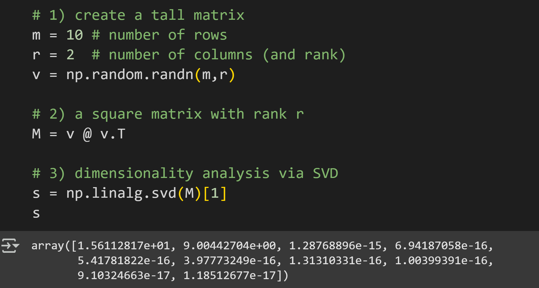
1. Here I create a 10x2 matrix of random numbers.

2. Multiply that matrix by its transpose. This is a trick in linear algebra to create a square symmetric matrix with a known rank. The rank of a matrix is similar to its effective dimensionality, although the rank includes small amounts of noise and rounding errors. The resulting matrix (variable M) will be a 10x10 matrix with rank=2. The theory and proof for why that is the case is not hard to understand, but it does require some background in linear algebra.

3. Here I extract the singular values via the numpy svd() function. That function returns three outputs, corresponding to the three SVD matrices that I showed in Figure 2. For our purposes, we only need the second output (the singular values), hence indexing [1] at the end.

The singular values printed out are curious. Centuries of math theory tells us that the first two singular values must be non-zero and rest must be exactly zero. And yet there are no zeros in that vector of singular values.

Don’t worry though; the math isn’t wrong. The issue is that computers have tiny rounding errors on the order of 10^{-15}. Those numbers should be zero but computers aren’t perfect. Therefore, we use a threshold to consider tiny numbers to be zero. The numpy developers know all about this problem, and that’s why they use a threshold (called a tolerance) to exclude tiny dimensions.

An effective dimensionality analysis is exactly the same idea! We just set the tolerance parameter in a different way. It works like this:

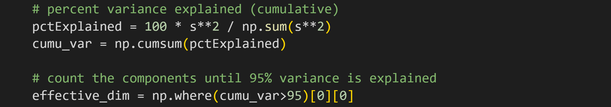
The code above converts the singular values to percent variance explained, calculates the cumulative sum, and finds the number of components it takes to explain 95% of the variability in the matrix. (There is a mostly inconsequential ambiguity about whether to take the component before or after the threshold; that will change the effective dimensionality by one, which doesn’t affect comparisons across different matrices.)

Let’s look at the results! Figure 4 below shows the matrix on the left, its “raw” singular value spectrum in the middle, and the singular values converted into cumulative percent variance explained on the right.

Figure 4: Visualization of a matrix and the procedure for finding effective dimensionality. The plot of singular values (middle panel) is called a “scree plot” in statistical parlance.

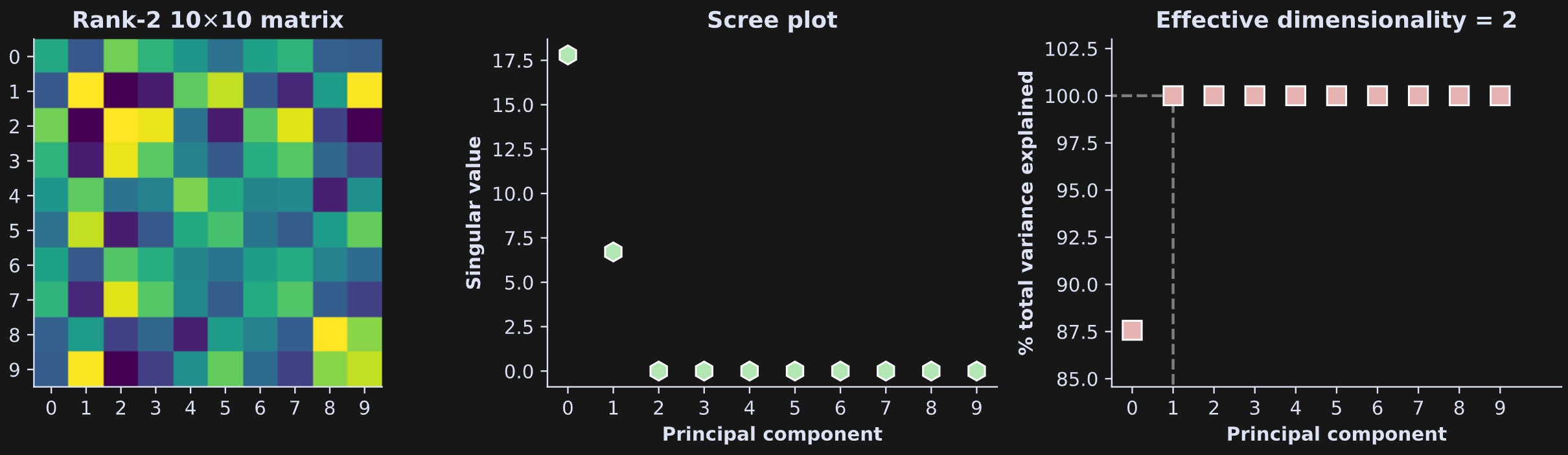
The cumulative plot on the right tells us how to interpret the raw singular values: The first component accounts for around 87.5% of the variance, the second component accounts for 100-87.5=12.5% of the variance, and the rest of the components account for none of the variance (precision errors notwithstanding).

In this example, the effective dimensionality equals the rank (2). That is a trivial result in this case.

Let’s see another, less trivial, example. In Figure 5 below, I ran the exact same code but changed the rank (the number or rows in the tall matrix) from r=2 to r=8.

Figure 5: Same as the previous figure, but with a rank-8 matrix.

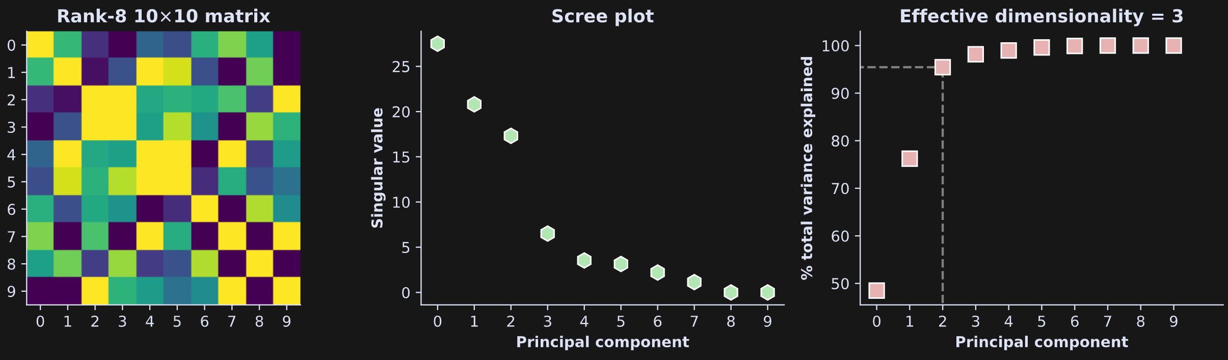
The singular values still taper down towards zero, but only the last two values (components 8 and 9) are actually zero; the first 8 are non-zero.

How is it possible that the effective dimensionality is only 3? That’s due to the difference in thresholding: I defined the effective dimensionality as 95% of the variance. Notice in the raw singular values plot (middle panel) that the top three components have large values and the next five are relatively small. Changing the threshold from 95 to 99 increased the effective dimensionality to 6 (not shown here but you can do it in the online code). This shows that the interpretation of effective dimensionality is impacted by the threshold parameter.

Demo 1: Dimensionality analysis in GPT2-XL

Now you know how dimensionality analysis works; it’s time to apply it to real data in a real language model.

For this demo, I’ll use GPT2-XL. It has 1.5 billion parameters — small enough to be convenient to work with, but big enough that we can find some interesting trends in a laminar profile analysis (that is, examine how the results vary over the 48 transformer blocks).

If you’re unfamiliar with the transformer block and the hidden states of an LLM, you might consider reading Part 4 of my 6-part series on using machine-learning to understand LLMs (actually, I recommend reading the entire series, but Part 4 is the most relevant to this post you’re reading now).

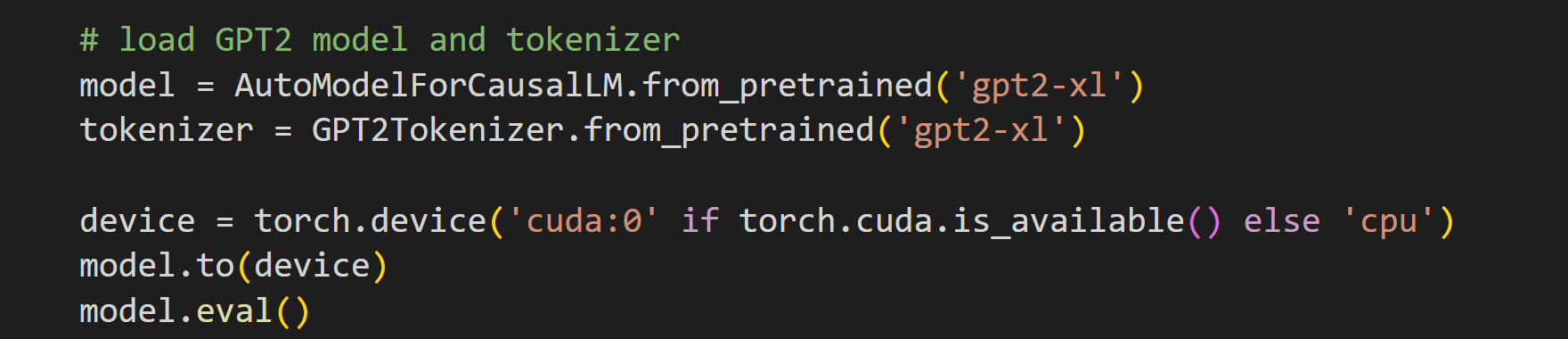
I’ll start by importing the model. If you have access to a GPU, then I recommend using it. No big deal if you’re using the CPU; this demo takes a few seconds to run on the GPU and a few minutes on the CPU. Start by importing the model, pushing it to the GPU, and switching the model to evaluation mode (that switches off some regularizations and other operations that are only relevant for training).

Analyses like effective dimensionality reflect model dynamics, not fixed model weights. That means we cannot perform this analysis on the model itself; instead, we need to do a forward pass with text and then analyze the model’s internal activations.

The text data I’ll use here is part of the book Through the Looking Glass (a.k.a. Alice in Wonderland). That book and myriad others is freely available on gutenberg.org.

The code extracts 1024 tokens from the text (1024 is model.config.n_ctx, which is the context window, or maximum sequence length). I excluded the first 10k tokens to get the actual book text and not the preamble. Here’re the first 100 tokens in the dataset:

 stay!” sighed the Lory, as soon as it was
quite out of sight; and an old Crab took the opportunity of saying to
her daughter “Ah, my dear! Let this be a lesson to you never to lose
_your_ temper!” “Hold your tongue, Ma!” said the young Crab, a little
snappishly. “You’re enough to try the patience of an oyster!

I’m also going to use the same tokens after randomly shuffling them. That is, the model will see the exact same tokens, but in a randomized order. It’s analogous to the difference between “I went to the store to buy chocolate” and “to go store buy I chocolate went the.” Same words, different order.

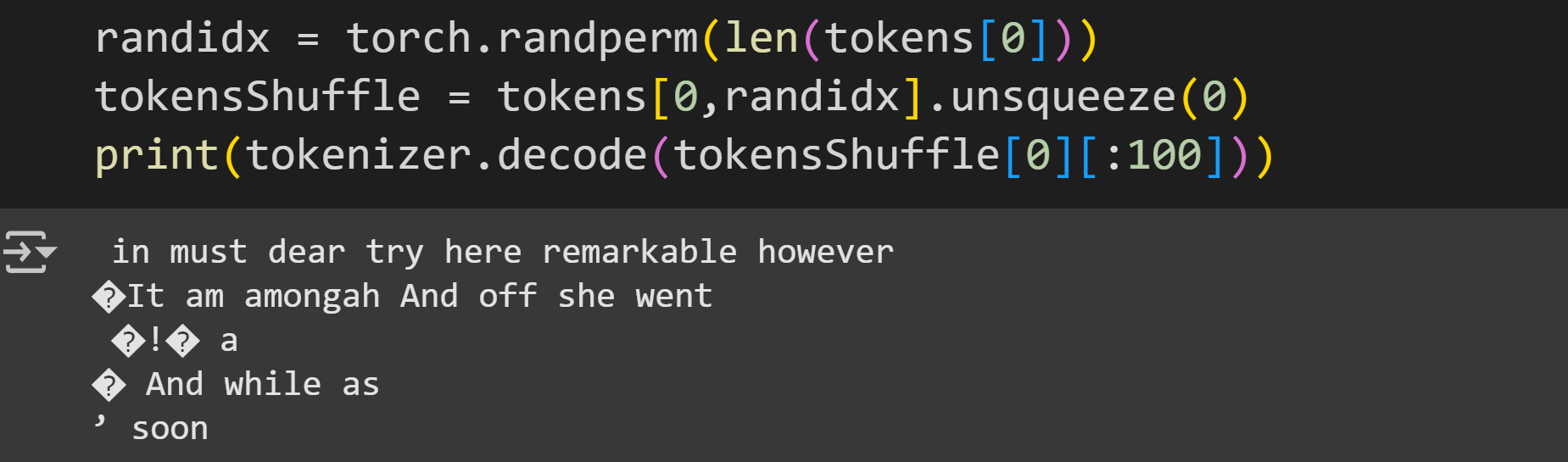
The reason to use shuffled tokens is to determine whether the results from the dimensionality analysis are due to the tokens per se, or to the patterns in the token sequence that the model extracts. That is, if the results of the dimensionality analysis are the same in the intact and shuffled inputs, then the effective dimensionality reflects a collection of tokens; on the other hand, divergent results indicates that the model is sensitive to the order in which the tokens appears.

The code below pushes the tokens through the model (after moving the tokens to the GPU) with different model outputs. The argument output_hidden_states gives us the output of all 48 transformer blocks (plus the initial embeddings vectors).

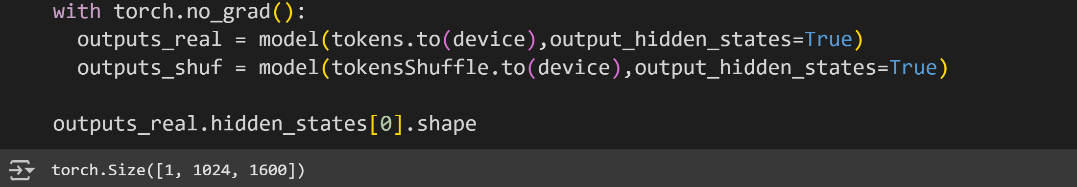
The hidden states are of size 1x1024x1600. That corresponds to one text sequence in the batch, 1024 tokens, and 1600 embeddings dimensions (check Part 3 of my LLM series for an explanation of embeddings dimensions). There are 49 tensors of the same size in the hidden_states list, one for each transformer block and one for the initial embeddings vectors. (btw, that code block is what takes a few seconds on a GPU vs. minutes on a CPU.)

Our goal now will be to apply SVD to each of those matrices, count the number of components to account for 95% of the total variance, and then plot the results.

Here’s what the code looks like. Please take your time to understand it before reading my explanation below.

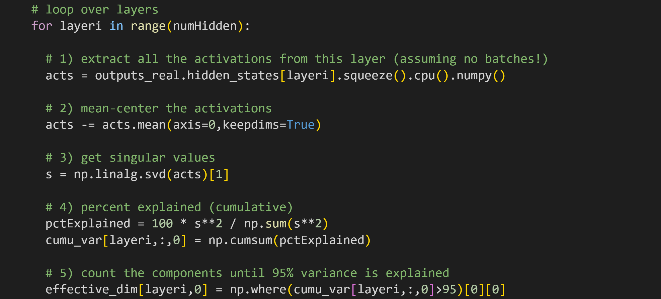
1. Numpy is not developed for GPUs, so we need to detach the activations tensor from the model’s computational graph, bring it back to the CPU, and convert from PyTorch to numpy format (PyTorch does have an svd routine, but numpy format is also convenient for subsequent data processing and plotting). The squeeze() method removes the first singleton dimension of the tensor to give us a matrix, which is necessary for the SVD.

2. Mean-centering a dataset means to subtract the mean so that the average of each vectors is zero. That’s important for PCA and effective dimensionality analyses, because global shifts in the data introduce biases in the SVD.

3. The SVD, just like I showed in Demo 0.

4. Convert to percent variance explained, and then to cumulative variance explained.

5. Effective dimensionality analysis, defined as the number of components it takes to account for 95% of the total variance in the internal activations for this transformer block (hard-coded here but it’s soft-coded in the code you can easily adjust the threshold). Remember that the singular values come out sorted descending, such that the largest values are always in the beginning of the vector.

And that’s all there is to the analysis! In the code file, the lines above are repeated for the shuffled tokens.

Before showing the results, I want to show a scree plot and cumulative variance explained, same as in Demo 0 but for real data, from transformer block 5 (out of 48).

Figure 6: Similar to Figure 5 but for real LLM activations data.

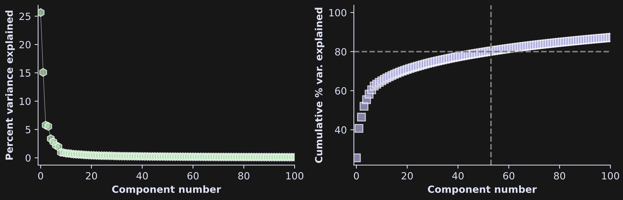
In this particular example, there are four components that each explain more than 5% of the variability. That’s out of 1024 components in total! Nonetheless, it takes several hundred more components to get up to 95% of the total variance. In fact, I drew the dashed lines in the right-hand plot at 80% variance so that you could see the rapid rise on the left.

What does this result tell us? For one thing, there are two large components and the rest are relatively small. On the other hand, those two components combined only account for around 40% of the variance, which means that the majority of the information in this transformer block is distributed over many small directions. We can speculate that this reflects the model incorporating multiple diverse pieces of context from other tokens when adjusting the embeddings vectors to generate an appropriate next token.

That’s for one transformer block. Figure 7 below shows the same result for all the transformer blocks, and for the real (left) and shuffled (right) tokens. In the plots, each line corresponds to the cumulative variance explained for one layer, color-coded such that higher numbers (towards yellow/red colors) correspond to transformers that are deeper into the model.

Figure 7: Cumulative explained variance for different layers in GPT2-XL. Dashed gray line corresponds to 95%.

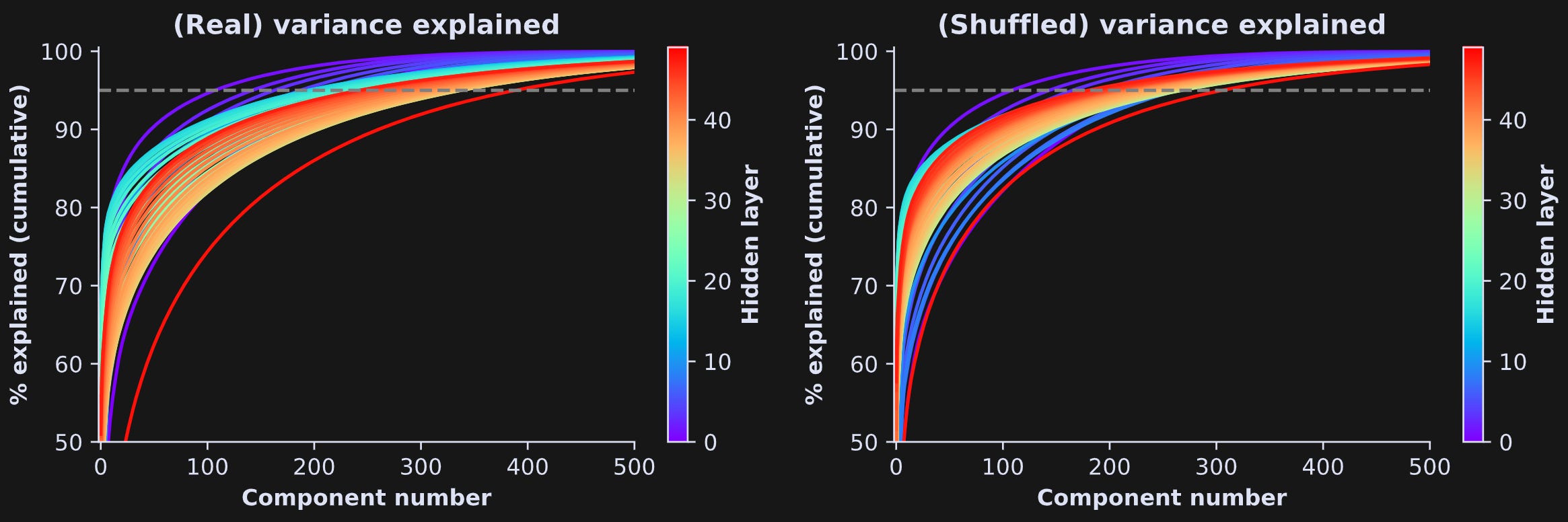
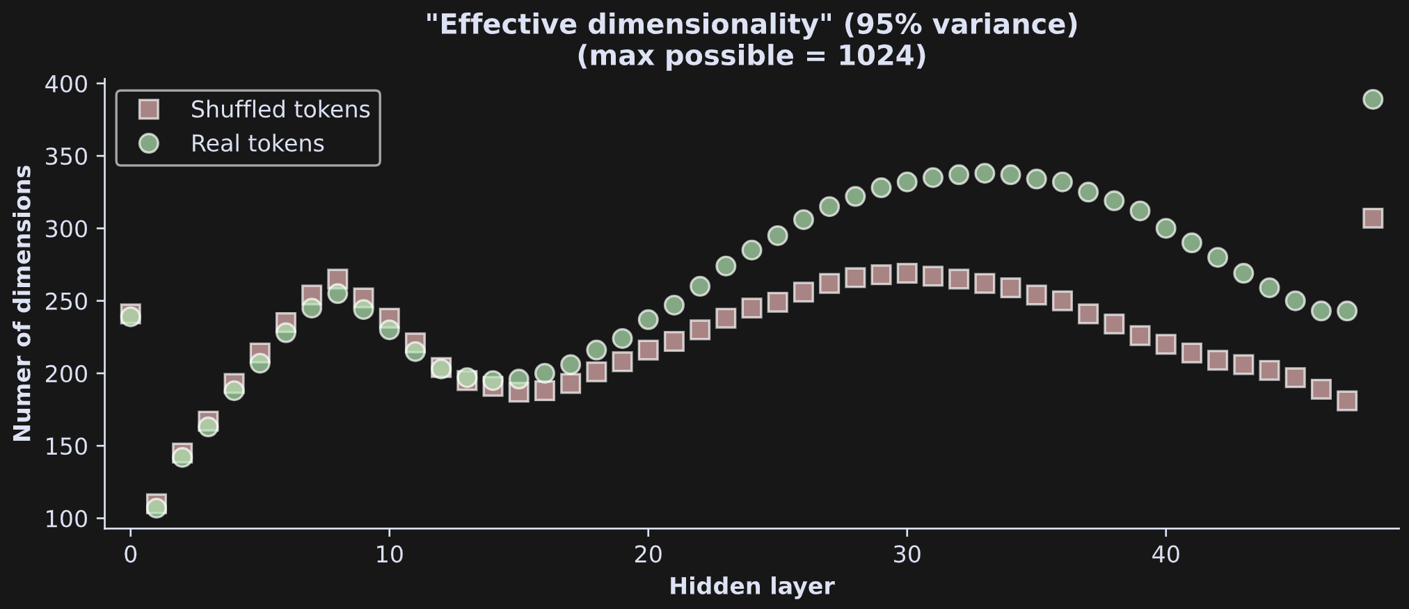
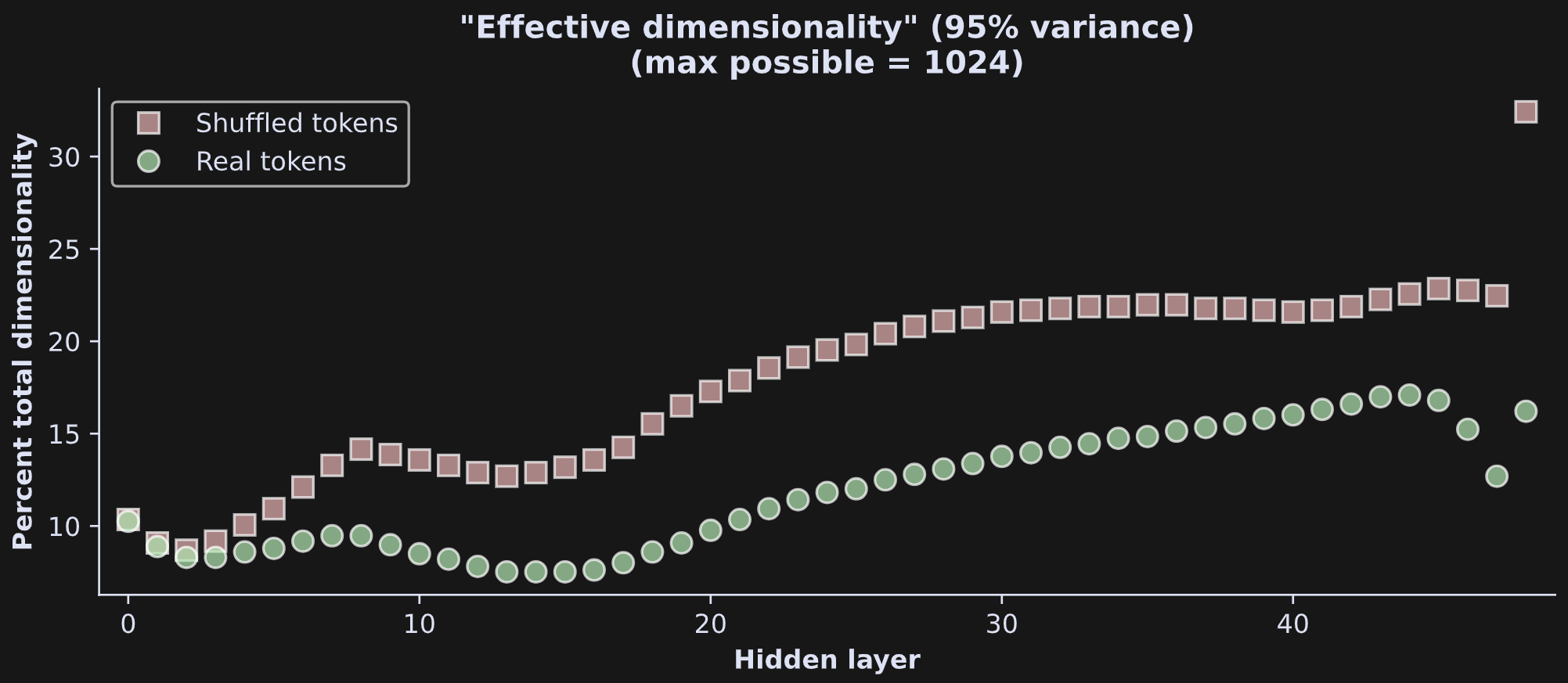
All layers have a similar “bending” shape reminiscent of a log transform, with the amount of bending varying across layers. From a rough eyeball estimate, it looks like the effective dimensionality ranges from 100 to 350, though that also varies quite a bit across layers. Figure 8 below shows the effective dimensionality in a scatter plot.

Figure 8: Laminar profile of effective dimensionality for the real tokens (green circles) and shuffled tokens (red squares). The first hidden layer is the initial token embeddings (no transformers applied), and the final hidden layer includes an additional normalization.

I find these kinds of results really interesting and thought-provoking. A few observations:

• The embeddings vectors are mostly contained in <350 dimensions. Is that a lot or a little? 300 dimensions seems like a lot, but the maximum possible dimensionality is 1024 (the maximum possible dimensionality is the smaller of the number of tokens or the number of embeddings dimensions). That means that only around a quarter to a third of the total available space in the model is occupied. What is the rest of that space doing?

• That said, keep in mind that 95% variance explained is an arbitrary threshold. The other 5% of the dimensions may be small in terms of how much variability they contain, but that doesn’t mean they are useless or uninformative. Indeed, very small pieces of information can have big effects.

• The first hidden layer (token + position embeddings) has relatively high dimensionality. There are no adjustments or contextual information that are brought into the embeddings at this layer, so it is qualitatively distinct from the rest of the model.

• The final layer of the model is a transformer block just like the preceding 47 transformer blocks; however, the hidden states output includes an additional layernorm normalization that clouds the interpretation.

• The transformer blocks show an interesting alternating pattern of increased then decreased dimensionality, reflecting transitions in how the model processes and contextualizes information. Smaller effective dimensionality suggests that the model has achieved a compacted representation of the tokens, i.e., that the patterns and structure in the text have been integrated to represent the same information in a smaller space. Subsequent increases in dimensionality reflect the model bringing on additional context and world knowledge that was not present in the original tokens.

• The real and shuffled token sequences have comparable dimensionality earlier in the model, and diverge around half-way through. The intact sequence allows the model to bring more world-knowledge into play, which requires additional complexity and processing space.

That list of observations should not be taken as grand conclusions about how all LLMs operate; it’s just one result from one model and one piece of text. A more rigorous investigation would involve more texts and more models. (In fact, this pattern is reproducible across multiple texts and GPT2 models, which I show in my full-length online course on LLM mechanisms.)

These observations are also based on a threshold of 95%. But the results are qualitatively the same when using a 99% threshold (not shown here but you can explore it using the online code).

Demo 2: Same analysis, different text data

Although the pattern of results in Figure 8 is similar in several texts that I’ve tried, there are other kinds of text data that LLMs have been trained on, for example, html and css code.

To explore possible differences in effective dimensionality, I re-ran the code file, but with a different source of text. This time I used the html/css code that powers this interesting website:

Figure 9: Yep, that’s a real website. And nope, I have no connection to, or affiliation with, that website or the organization behind it.

Here’s what a snipped of raw website code looks like:

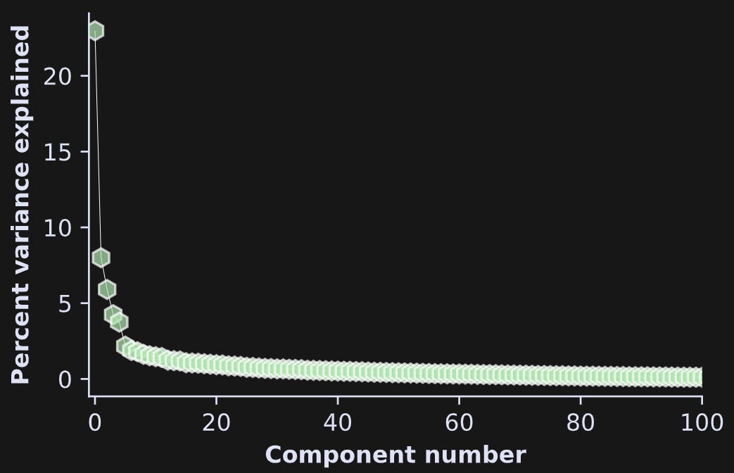
etype');}@font-face {font-family: 'Open Sans';font-style: normal;font-weight: 400;font-stretch: normal;font-display: swap;src: url(https://fonts.gstatic.com/s/opensans/v43/memSYaGs126MiZpBA-UvWbX2vVnXBbObj2OVZyOOSr4dVJWU

Figure 10 below is the same as the left panel of Figure 6, but with html code instead of text. Notice that the spectrum is more dominated by a single component, compared to Figure 6.

Figure 10: Scree plot of the 5th transformer block when using html code instead of Through the Looking Glass.

And Figure 11 below shows the laminar profiles of effective dimensionality. Some features are comparable to the plot earlier with the English text, but overall I’d say that this result looks quite distinct.

Figure 11: Effective dimensionality analysis when processing html code.

The end of this post — but the start of your journey into LLMs!

There are two conclusions I’d like to draw from this post:

1. Applying machine-learning techniques to LLM data is a fun and powerful way to explore and understand how LLMs are put together and how they process text. There is a newly emerging field of mechanistic interpretability of LLMs. That field is relevant for understanding complex systems and emergent behaviors, and is foundational for technical AI safety.

2. Substantively, it is difficult to draw grand conclusions from small-scale experiments like what I showed here. There are some features of model dynamics that are preserved across models and dataset types, and there are other features that are distinct. That doesn’t mean we can learn nothing about LLMs; it does mean that research on large complex systems is challenging for multiple reasons, and that rigor and meticulous experiments with a variety of datasets and models is important.

Help increase my effective dimensionality

I hope enjoyed this post! I wrote it during “business hours” because this is my business. I can afford to make this my business because last month, some very kind people enrolled in my courses, bought my books, and/or became paying subscribers here on Substack.

If you would like me to continue creating high-quality affordable education next month, then please consider doing the same. If your budget is tight, then please just share my links and use your money for more important things.

Video explanation of code and results

The video below is for paid subscribers. It is a 20-minute discussion of the code and the analyses, with some deeper explanations of the code implementations and findings.