Confidence intervals 1/3: interpretation and equation

Start building confidence about confidence intervals in the first of this three-part series.

About this three-part series

Welcome to the first part of the series! By the end of the trinity of posts, you will understand how to use, interpret, and calculate confidence intervals (ahem, I am confident that you will increase your confidence about confidence intervals.)

I like to use code to help teach data science, because you can learn a lot of math with a bit of code. However, only the essential code bits are shown in the post, and the full code files that will reproduce the figures and that you can adapt for your own analyses, are on my GitHub page.

Here’s the link! I encourage you to run the code (and adapt it!) as you’re reading this post.

And here are the links to post 2 and post 3.

What is a confidence interval and what is it used for?

How tall is the average adult male in Uzbekistan?

I don’t know, but I do know that if we want The True answer, we would need to measure the height of every adult male in Uzbekistan, even those who died centuries ago and those who haven’t been born yet. That’s just… infeasible.

So instead, we can measure a sample of adult Uzbeki men, and if that sample is random (meaning every adult male currently alive has an equal chance of being measured), then we can say that the sample average is an approximation of the true average.

But how good is that sample average? That is, how confident can we be that the sample characteristic is close to the true population parameter?

Enter the confidence interval.

Confidence intervals (abbreviated C.I. or CI) are an insightful yet underutilized metric in statistics. I suspect that many data scientists don’t use CIs because they are unsure how to calculate and interpret them. I hope this three-part series changes that for you :)

There are two applications of confidence intervals in data science:

1. To estimate bounds on a statistical parameter. A CI provides bounds around the sample average that tell us about the precision of that estimate. Sometimes a 95% CI is interpreted as indicating that you can be 95% confident that the population average is within the CI bounds around the sample average. However, that is not entirely accurate. Instead, a 95% CI indicates that if we were to collect a large number of samples from the same population, 95% of those samples would have confidence interval bounds that include the true population average.¹

2. To evaluate statistical significance. Here the idea is that if the null hypothesis value is outside the CI bounds, then the effect is considered statistically significant. For example, if a sample average is .5 with 95% confidence interval bounds of [.1,.9], then we can say that the average is statistically significantly different from zero at a confidence level of 95%, which corresponds to α = 5%.

For both of these applications, small CIs are generally better, because they indicate higher-quality data with more precise estimates of the population average.

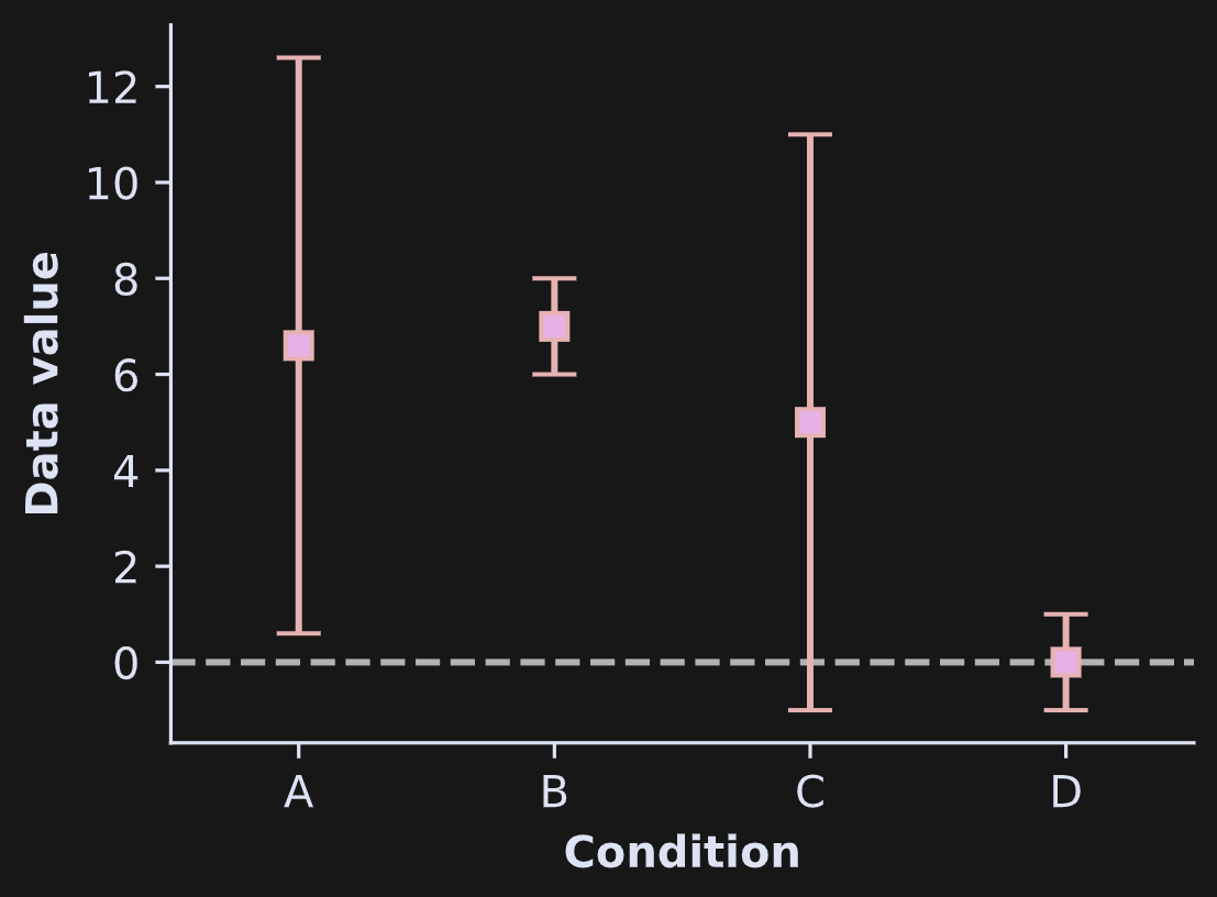
Confidence intervals are visualized either as bars or as shaded areas. In Figure 1, imagine that the boxes in the plot show the averages in each group, and the error bars indicate 95% confidence intervals. If the horizontal dashed line is the null-hypothesis value of no effect, then groups A and B would be significantly greater than zero while groups C and D would not be.

Figure 1: Confidence intervals, visualized.

Where do confidence intervals come from?

Confidence intervals are calculated in one of two ways:

1. Analytically (based on a math equation). This works only for certain statistical analyses and is based on some assumptions. You’ll learn the analytic formula for the average in this post.

2. Empirical (based on bootstrapping). This method works for many statistical analyses, including analyses that have no analytic CI or data that violate the assumptions. You’ll learn about this method in Part 2 of this series.

Here’s the formula for the confidence interval around the sample average:

The x with a bar over it (Substack doesn’t have inline latex capabilities…) is the sample average, s is the sample standard deviation, n is the sample size — and by the way, that fractional term is also known as the standard error of the mean, SEM — and the t* is a t-value. It’s not a t-statistic from a t-test, but it does come from a t-distribution. It is the t-value that corresponds to 5% of a t-distribution with n-1 degrees of freedom. 5% corresponds to a 95% CI.

Let’s reflect on that equation. Remember that we want small CIs around the average. The formula tells us that there are two ways to shrink the confidence interval: decrease the numerator (s) or increase the denominator (n). The standard deviation decreases when the data are more homogeneous (all the data points are close to the mean), and the sample size increases… well, it increases when you have larger samples.

These factors are not always trivial to control in actual research, especially if the data are already collected. But you can improve the situation through data cleaning, which you will see in Part 3 of this series!

One major advantage of analytic CIs is that you don’t need raw data; you only need the mean, standard deviation, and sample size. That means you can calculate CIs of any study published at any time in history — as long as the authors reported those three sample characteristics.

Here’s how you’d translate that equation into code:

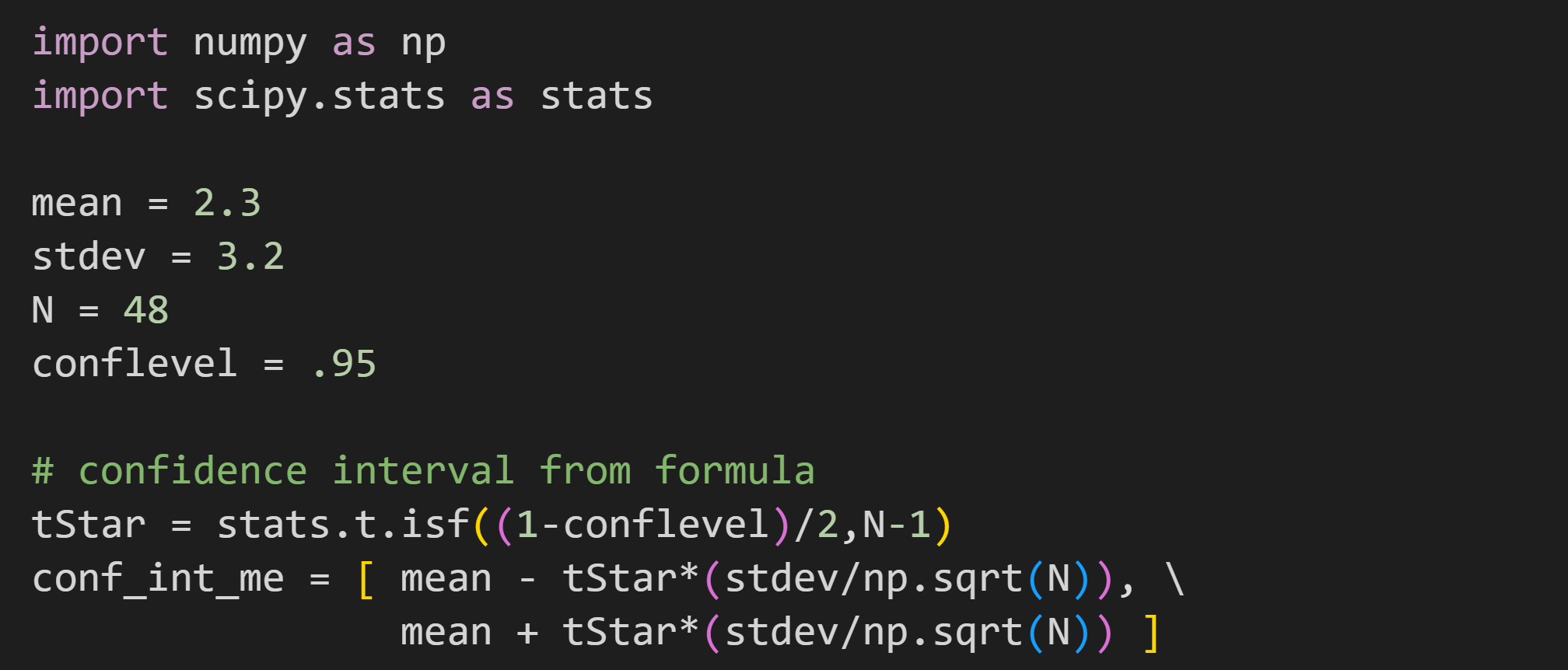
With those numbers, the 95% CI around the mean is 2.3±.93.

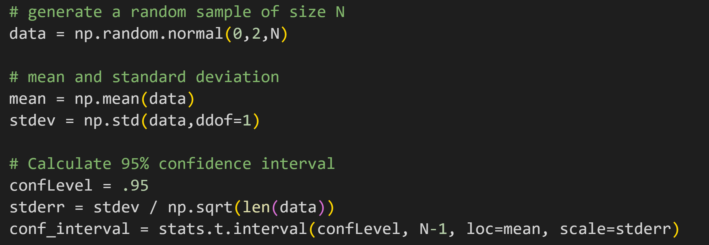
Although it’s instructive to see math translated into code, in practice its better to use the interval method that the scipy developers worked so hard to create:

Assumptions of analytic confidence intervals

Ah yes, the pesky assumptions. Statistical analyses based on math formulas (“parametric statistics”) are valid only when assumptions are met. Fortunately, most of the assumptions are the same for all parametric analyses, so the list below will probably look familiar.

1. Random sampling. Each member of the population should have an equal chance of being included in your sample. For example, if you want to know the average retirement investment amount among Irish 40 year olds, your sample (and, therefore, the CI around the sample average) will be biased if you only survey people living in Dublin.
   Random sampling is also related to independence. If you collect each new data sample by getting a friend of the previous sample, then those samples are dependent on each other.

2. Large enough sample. There is a lot of variability in the world, and so a very small sample size might not be representative of the population just by chance (sampling variability). How large of a sample is large enough? Well, that’s difficult to say because it depends on the effect you’re measuring. Appropriate sample sizes can be estimated using formulas, but in general, the more variability in the data, the larger the sample size should be.
   There is also a more technical reason for large sample sizes: The CI formula is based on the Central Limit Theorem, which only kicks in for larger sample sizes. But again, there is no magical minimum sample size, because the Central Limit Theorem can work really well even in samples of 5 if the data are normally distributed.

3. Homogeneity of variances. If you are working with multiple groups (for example, a group of patients and a group of controls in a medical study), then all the groups should have the same standard deviation.

Do your data violate these assumptions? It might not be so bad. Parametric statistics like analytic CIs tend to be “reasonably robust” to “minor violations” of assumptions. I use apology quotes there, because “reasonable” and “minor” are difficult to quantify. There are statistical methods to determine if your data have strong violations, which I won’t go into in this post.

But even if the assumptions are strongly violated, then fear not, dear reader! CIs based on computational statistical procedures like bootstrapping don’t depend on most of these assumptions. More on that in Part 2!

Is CI the same as standard deviation?

Nope! They are conceptually related to each other, in that they are both measures of variability. But they are distinct. Here’s an overview of each measure, and then I’ll discuss their differences.

• Standard deviation. Standard deviation measures the amount of variability within a dataset, defined as the average squared distance between each data point and the mean. A small standard deviation indicates that the data points are close to the mean, whereas a high standard deviation indicates that the data points are spread over a wider range.

• Confidence interval. CIs provide bounds within which we expect the population parameter to be, in repeated samples from the same population. The wider the CI, the more uncertainty there is about the estimate.

Here are the key differences:

• Standard deviation is a measure of variability within one sample, while a CI provides a range that we expect the population parameter to fall into in future samples.

• Standard deviation provides information about the spread of individual data points around the mean, while CIs provide an uncertainty estimate of the true population mean.

• CIs take sample size into account, while standard deviation does not. To clarify: The standard deviation formula (not shown here) includes the sample size, but increasing the sample size does not impact the standard deviation (although it is more reliably estimated with larger sample sizes).

Let’s run a code demo to explore the distinction between CI and standard deviation. The idea is to simulate two datasets, one small (N=50) and one large (N=2000) and calculate their standard deviations and 95% CIs.

(Reminder that only the essential code is printed in this post; you can get all of the code from my GitHub.)

I put that code into a for-loop over the two different sample sizes (variable N), and added some additional visualization code to produce Figure 2.

Figure 2: Data distributions (gray bars), mean (thick white vertical line), standard deviations (green dotted line), and 95% CIs (red dashed line).

Notice that the means and standard deviations are the same for both datasets (well, not exactly the same because of sampling variability, but very similar) whereas the CIs are much tighter for the N=2000 sample. That should be intuitive: the larger the sample, the more confident we can be that the sample average matches the population average.

That’s for two samples; in the next analysis, I repeated that code over a larger range of sample sizes and stored the width of the standard deviation and CIs for each sample size (by “width” I’m referring to the distance between the two bars on either side of the average in Figure 2). Those results are shown below.

Figure 3: Standard deviation is unrelated to sample size while CI continues to decrease with increasing sample size.

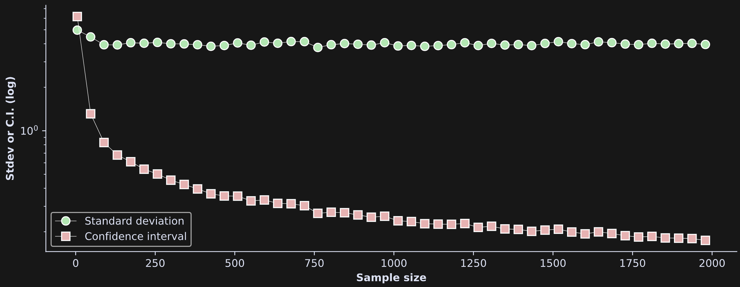
By the way: It is arbitrary that I used 1 standard deviation and 95% CI — why not .784 standard deviations and a 92.45% CI? These kinds of choices would change the y-axis values, but wouldn’t change the relationship to sample size.

---

And that’s it for Part 1! In Part 2, you will learn how to calculate CIs using computational statistics (bootstrapping), and then in Part 3 you’ll get to apply what you learned here to real datasets. Very exciting :D

Increase my sample size :P

I write these posts because I want to bring high-quality technical education to as many people as possible — but also because it’s my job and my source of income. Please consider supporting me by enrolling in my online courses, buying my books, or becoming a paid subscriber here on Substack. If you have a tight budget, then please keep your money for more important things, and instead just share these links.

1. For convenience, I’m only discussing CIs around the sample average; I’ll extend the discussion to other statistical characteristics in the next two parts.