Correlation vs. cosine similarity

What’s the difference between us? We can start at the... normalization

Height and weight, outdoor temperature and ice cream sales, exercise and health… there are myriad examples of relationships between variables. But how do you quantify those relationships?

There are many statistical analyses that quantify bivariate (two variables) relationships; in this post I will describe two — correlation and cosine similarity — discuss how they relate to each other, and advise you on when to use which one. The upshot is that the measures can be identical but are often different. Which one to use depends entirely on whether the scale of the data is important.

I’ll start with some math and explanations, then some cool Python demos that you can try yourself.

The dot product

But before getting to the measures, let’s start with the dot product. The dot product is one of the most important foundational operations in mathematics, certainly in applied math topics like data science and deep learning.

The dot product is a single number that captures the linear relationship between two variables. Mathematically, it is defined as element-wise multiplication and sum. Here’s a small example:

\(\begin{bmatrix}1\\2\\3\end{bmatrix} \cdot \begin{bmatrix}3\\-1\\0\end{bmatrix} = (1\times3) + (2\times[-1]) + (3\times0) = 3-2+0 = 1\)

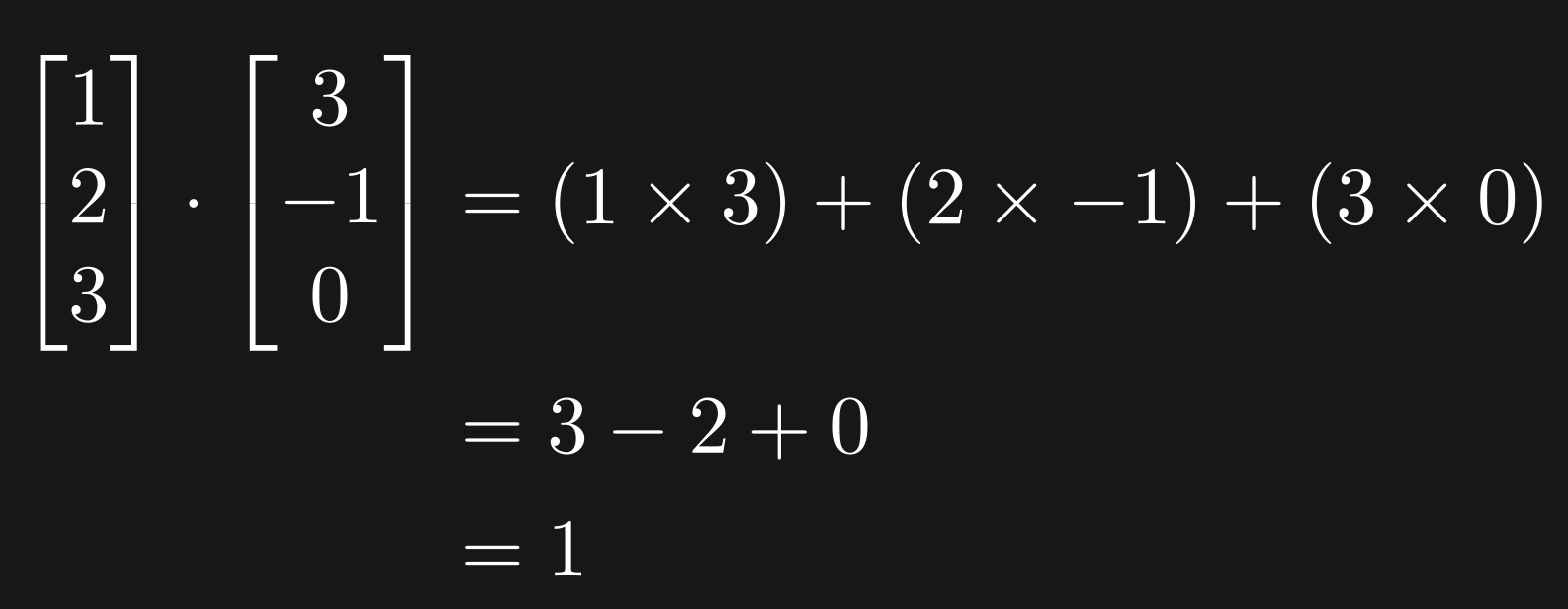
Needless to say, the two variables need to have the same number of numbers, otherwise they don’t pair off and the dot product calculation fails :(

What does the result mean? The “raw” dot product (“1” in this example) is difficult to interpret on its own, because it reflects a combination of (1) the scale of the first variable, (2) the scale of the second variable, and (3) the linear relationship between the variables. We want to isolate that third component, which means we need to normalize the dot product before interpreting it.

Two small comments: (1) The dot product is linear because it involves only summing and multiplying; there are no square roots, powers, logs, trig transformations, or other nonlinearities. (2) There is a geometric interpretation of the dot product, which I’m not going to discuss here.

Mathematically, the dot product between variables x and y can be defined like this:

\(\alpha = \sum_{i=1}^n x_iy_i \hspace{10em} (1)\)

In English: Element-wise multiply all n pairs of data points, then sum.

Pearson correlation: The doubly-normalized dot product

There are several types of correlation coefficients; Pearson is the most commonly used one, and when someone says “correlation” they’re almost certainly referring to the Pearson variety. Here’s the equation for a Pearson correlation:

\(r \;=\; \frac{ \sum_{i=1}^n(x_i-\overline{x})(y_i-\overline{y})}{\sqrt{\sum_{i=1}^n(x_i-\overline{x})^2\sum_{i=1}^n(y_i-\overline{y})^2}} \hspace{10em}(2)\)

r is the correlation coefficient, x and y are the two variables (e.g., vectors of height and weight values for a sample of people), n is the sample size, and the x with a horizontal bar on top is the average of x. Notice that the formula is a ratio of a dot product between x and y in the numerator, and two dot products in the denominator (the squaring makes it look different from a dot product, but you can write x^2 as x*x). Thus, the correlation is formed from dot products.

What does this equation mean? Let me start by explaining the two normalizations:

1. Mean-center. The variables are shifted by their average, such that the variables in the correlation equation have a mean of zero.

2. Variance-normalizing (denominator). The squared terms in the denominator are the variances of the variables. (Small nuance here: variance technically needs a 1/(n-1) term, but it’s in the numerator and denominator and therefore cancels.) Dividing by the product of the variances eliminates their scaling. Basically, the variance normalization accounts for the fact that, for example, weight has a different numerical value if we measure in grams, kilograms, stones, or pounds, even though the relationship between height and weight doesn’t depend on the measurement units.

Why do we need these normalizations? If you want to know the relationship between, for example, time spent in higher education and post-education salary, you don’t want to worry about whether “time spent” is measured using hours, days, months, or years; and you don’t want to worry about whether salary is measured using dollars, thousands of dollars, or hundreds of thousands of dollars. Instead, you just want to know whether the relationship is positive, and how strong the relationship really is. Without the normalizations, you’d get a different correlation coefficient depending on the measurement units.

Furthermore, imagine that the two variables are already mean-centered and unit-normalized; in that case the equation for the Pearson correlation would literally be identical to the dot product equation I showed earlier.

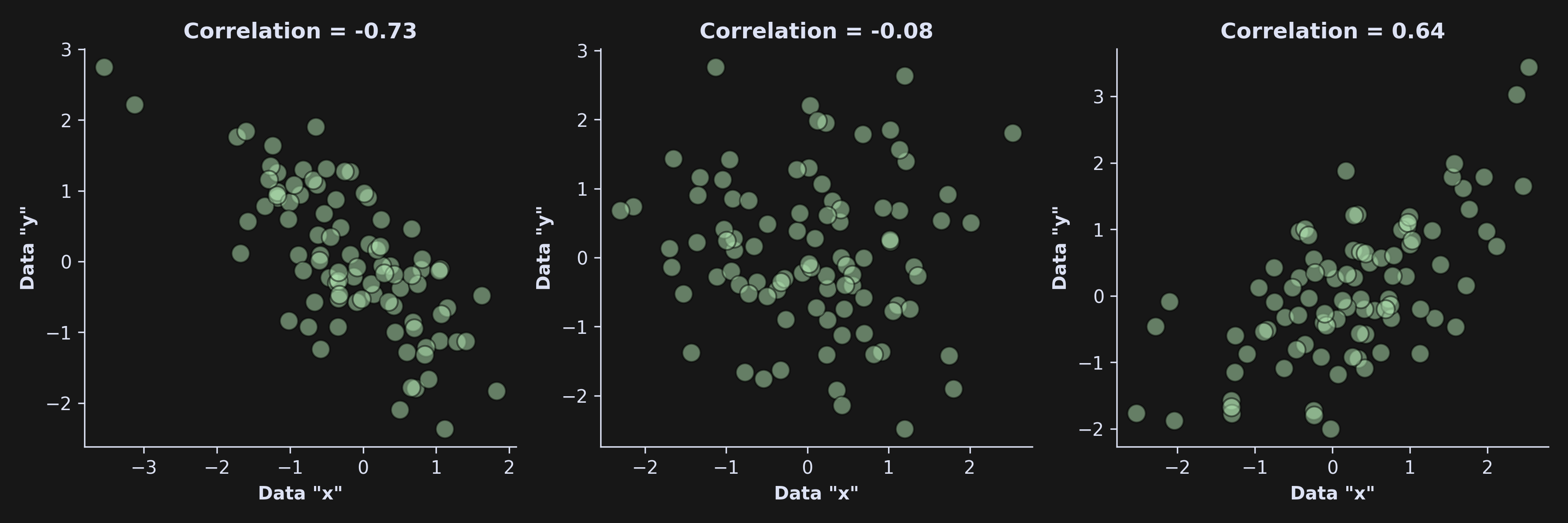
And what does the (suitably normalized) coefficient value mean? When the two variables are identical (that is, x=y), then r=1. And when the two variables are identical-but-opposite (that is, x=-y), then r=-1. When r=0, the variables are completely unrelated to each other (e.g., the price of Bitcoin vs. the growth rate of a bacteria deep in the Mariana Trench). For some intuition, here’s a picture of three datasets with three correlation coefficients:

Figure 1: Three datasets illustrating negative (left), negligible (center), and positive (right) correlations.

On the other hand, check out the correlation between x and y here:

Figure 2: These examples show that correlation analyses cannot capture nonlinear relationships.

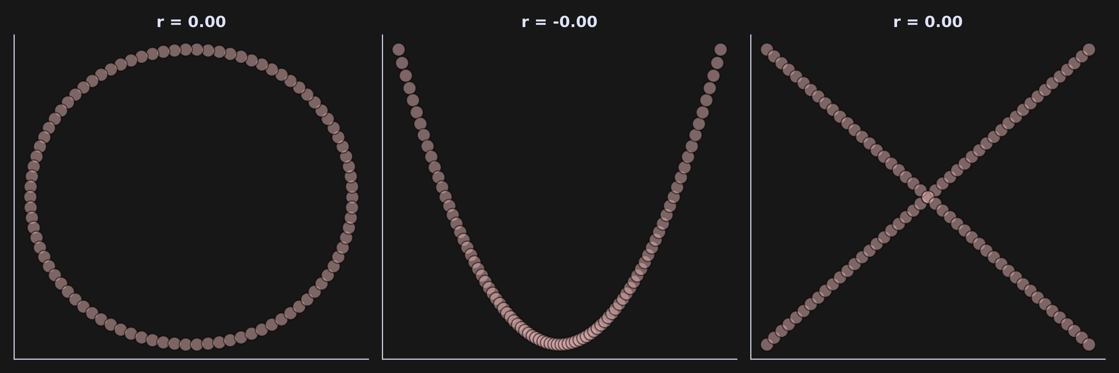
This demonstrates that correlation (and also cosine similarity!) can only measure linear relationships. Nonlinear relationships can be captured using, for example, mutual information. More on that in another post!

Cosine similarity

Now for cosine similarity. Cosine similarity (sometimes indicated Sc for “similarity of the cosine variety”) is the first Equation 3 below; I’ve repeated the correlation coefficient underneath (Equation 2) for ease of comparison.

\(\begin{align} S_c \;&=\; \frac{ \sum_{i=1}^nx_iy_i}{\sqrt{\sum_{i=1}^nx_i^2\sum_{i=1}^ny_i^2}} \hspace{10em}(3)\\\\ r \;&=\; \frac{ \sum_{i=1}^n(x_i-\overline{x})(y_i-\overline{y})}{\sqrt{\sum_{i=1}^n(x_i-\overline{x})^2\sum_{i=1}^n(y_i-\overline{y})^2}} \hspace{4.5em}(2) \end{align}\)

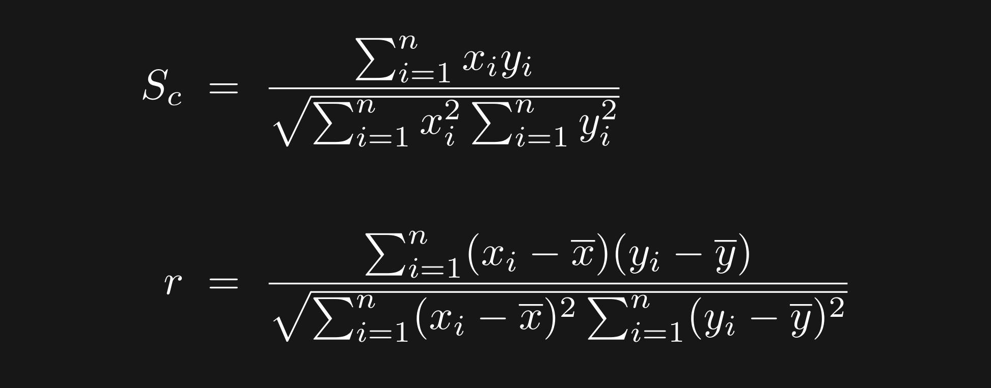
What would happen if x and y were already mean-centered? The two formulas would be identical. (As with correlation, there is a geometric interpretation that I’m not focusing on.)

In other words, correlation and cosine similarity can be identical. But what happens when the means aren’t zero? That is an intuition is that is really difficult to develop just by staring at formulas. So instead, let’s run some simulations in Python!

Code simulations to build understanding

Note about the code below: I’m only showing the most important lines of code; you can download the entire notebook file from my git repo. After reading through the rest of this post, I very strongly encourage you to play around with the code yourself.

Simulating correlated data

Before we get to the direct comparisons, you need to know how to simulate correlated data. That’s useful because it allows you to explore the relationship between correlation and cosine similarity with ground-truth data.

\(\begin{align} x &\in \mathcal{N}(0,1) \\ q &\in \mathcal{N}(0,1) \\ y &= xR + q\sqrt{1-R^2} \end{align}\)

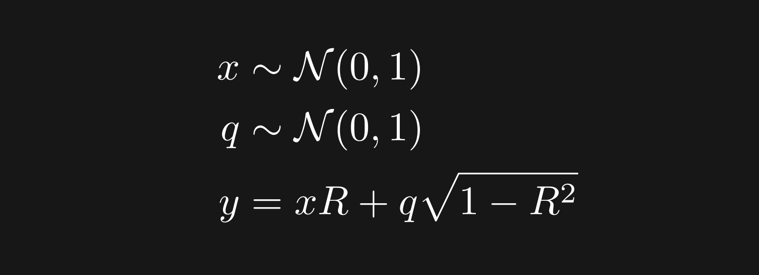
In other words, x and q are random numbers sampled from a normal (Gaussian) distribution, and x and y are variables correlated at approximately r=R. Why is the actual correlation only approximate? That’s because R is the population correlation while r is the sample correlation. With larger sample sizes, the sample correlation will more closely match the population correlation.

The way to think about the third equation is that y equals a copy of x that is scaled up by R, and then added to random noise scaled down by R. Notice what happens when R=0: y is simply random numbers, unrelated to x. On the other hand, when R=1, then y=x exactly.

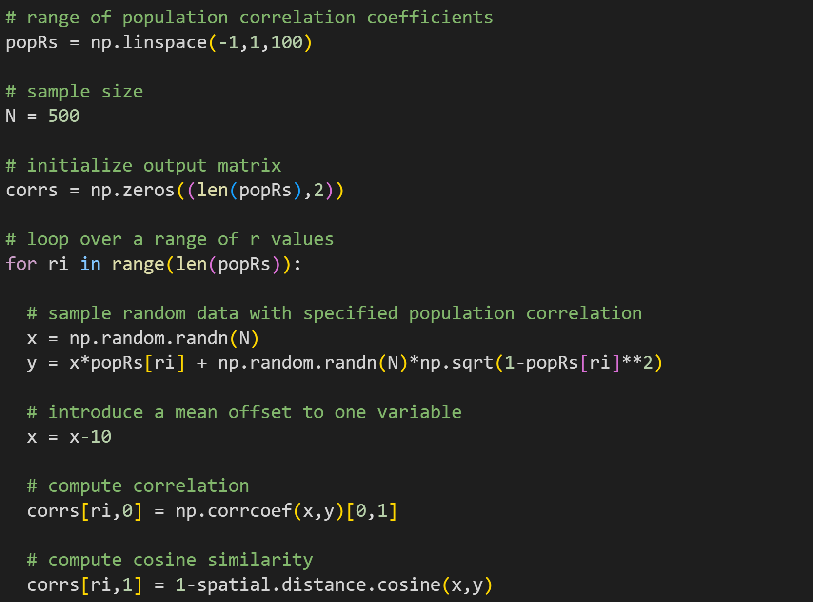
How’s this look in code? Something like this:

import numpy as np
import matplotlib.pyplot as plt

R = .7
x = np.random.randn(N)
y = x*R + np.random.randn(N)*np.sqrt(1-R**2)

plt.plot(x,y,’o’)

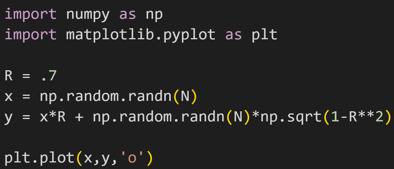
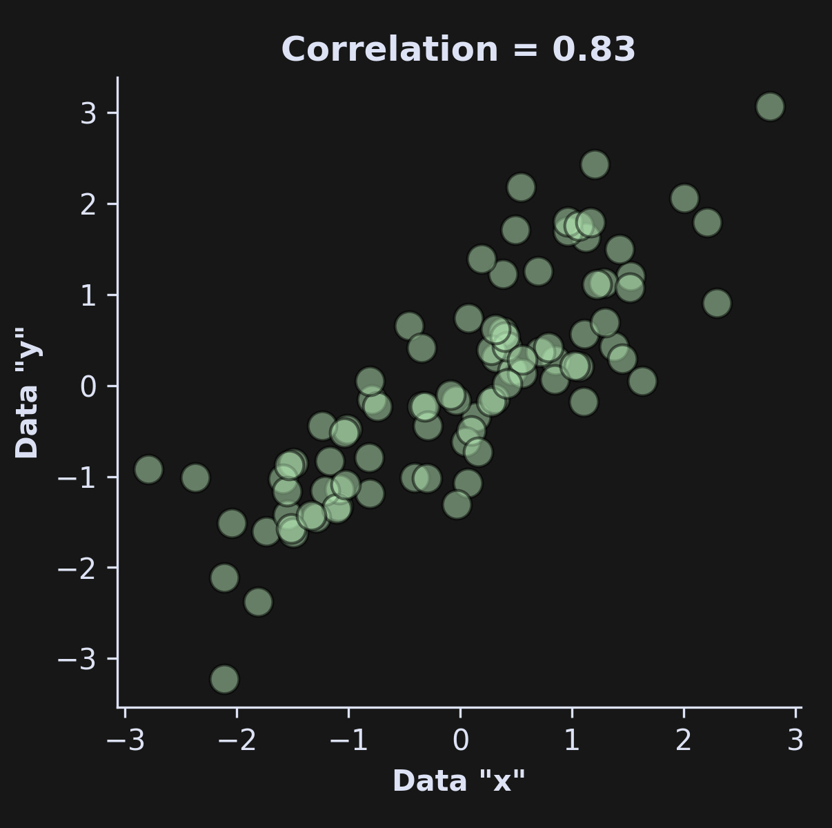
That produces a graph like this (reminder that the code snippet above is just the essentials; the full code is linked here):

Figure 3: Simulated random correlated data. Simulating data is a powerful way to learn data science.

Calculating correlations and cosines in code

The code block below shows how to calculate correlation and cosine similarity using a direct translation of the formulas shown earlier.

# Pearson formula
xnorm = np.sum( (x-x.mean())**2 )
ynorm = np.sum( (y-y.mean())**2 )
r = np.sum( (x-x.mean())*(y-y.mean()) ) / np.sqrt(xnorm*ynorm)

# compute cosine similarity
xnorm = np.sum( x**2 )
ynorm = np.sum( y**2 )
cs = np.sum( x*y ) / np.sqrt(xnorm*ynorm)

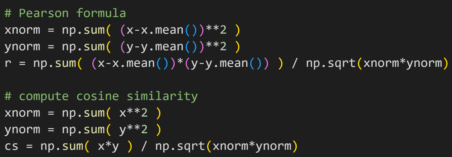
It’s useful to see the math translated directly into code, although in practice it’s better to use library-provided functions:

r = np.corrcoef(x,y)[0,1]
from scipy import spatial
cs = 1-spatial.distance.cosine(x,y)

Systematic comparison of correlation and cosine similarity

Now we’re ready for the experiment!

The goal here is to simulate correlated data, with correlation values ranging from -1 to +1. The data are created using the equation I showed earlier, but I added an offset of -10 to variable x. Of course, that doesn’t matter for the correlation because the mean is subtracted off. But that offset does get incorporated into cosine similarity.

# range of population correlation coefficients
popRs = np.linspace(-1,1,100)

# sample size
N = 500

# initialize output matrix
corrs = np.zeros((len(popRs),2))

# loop over a range of r values
for ri in range(len(popRs)):

  # sample random data with specified population correlation
  x = np.random.randn(N)
  y = x*popRs[ri] + np.random.randn(N)*np.sqrt(1-popRs[ri]**2)

  # introduce a mean offset to one variable
  x = x-10

  # compute correlation
  corrs[ri,0] = np.corrcoef(x,y)[0,1]

  # compute cosine similarity
  corrs[ri,1] = 1-spatial.distance.cosine(x,y)

And here’s what the results look like:

Figure 4: Divergence of correlation (red squares) and cosine similarity (blue circles), due to a mean offset in the data that is normalized-out in correlation. x-axis shows the ground-truth population correlation value.

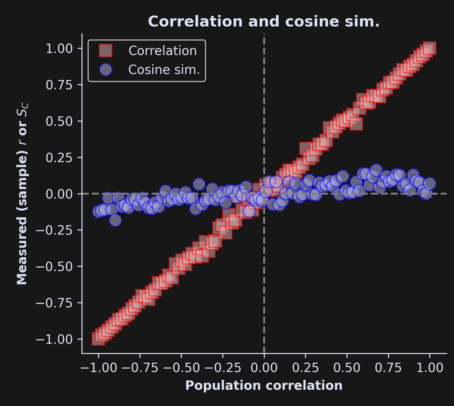
Stunning differences! The x-axis is the population correlation value (R) and the y-axis is the sample correlation (r) or cosine similarity. The correlation coefficient nearly perfectly tracks the population correlation, with minor deviations attributable to noise and limited sample sizes. The cosine similarity, on the other hand, remains quite small, regardless of the actual correlation coefficient. That discrepancy is entirely due to the mean offset in variable x.

Importantly, neither analysis is inherently “right” or “wrong”; they’re simply different. Now, these simulated data are meaningless, so it’s not possible to say which analysis is more appropriate in this example. But it is super-duper clear that you can get very different results.

If you want to continue exploring the code — which I super-duper recommend — then some suggestions are to (1) change the value of the x offset, (2) include a y offset that matches the x offset, (3) include a y offset with the opposite sign as the x offset.

When to use which?

Briefly:

• Use correlation when you want to measure the relationship without the worrying about the units. That’s the case when the units are arbitrary (e.g., distance can be measured in feet or meters) or different (e.g., euros vs. calories).

• Use cosine similarity when both variables have the same units — and the units are informative. Cosine similarity is often used in machine-learning applications with vector-embeddings, for example of text documents or tokens in a language model. In these cases, offsets between the variables correspond to meaningful differences, and thus really do indicate weaker relationships.

The end… of the beginning

There’s so much more I could write about bivariate relationships, in data and in real life… but I’ll stop here.

If you want to support me so I can continue spending my time educating you and others, then please enroll in my online courses, buy my books, or check my github page. I try to make my courses and books affordable, but if money is a limitation, then I’m grateful that you shared this post with your friends, colleagues, arch-enemies from middle-school, grandma’s bridge club, etc.