
EEG synchronization workshop part 2: optimal multivariate spatial filters
Learn neuroscience EEG signal processing and brain connectivity analyses

Hi again!
This is post 2 of a two-post series on an EEG synchronization analysis workshop I gave in October 2025.
Here’s the link to post 1.
If you are reading this but haven’t read post 1: If you’re already familiar with the Fourier transform, time-frequency analysis, and phase synchronization, then it’s probably fine to start with this post. But keep in mind that this post relies on knowledge that I taught in post 1, so if you start with this post but get confused about the signal processing aspects, then I recommend going through the first post first.
Getting the code and data
If you went through post 1, then you already have all the code and data files you’ll need for this post.
As a reminder: Each section below has its own code file. You can get all of the code files from my GitHub repo. Post 1 has a short video about downloading the code.
Deliverables from this post
By the end of this post, you will create the following figures in MATLAB. What do those figures mean and how do you create them? You have to watch the videos in this post to find out :P
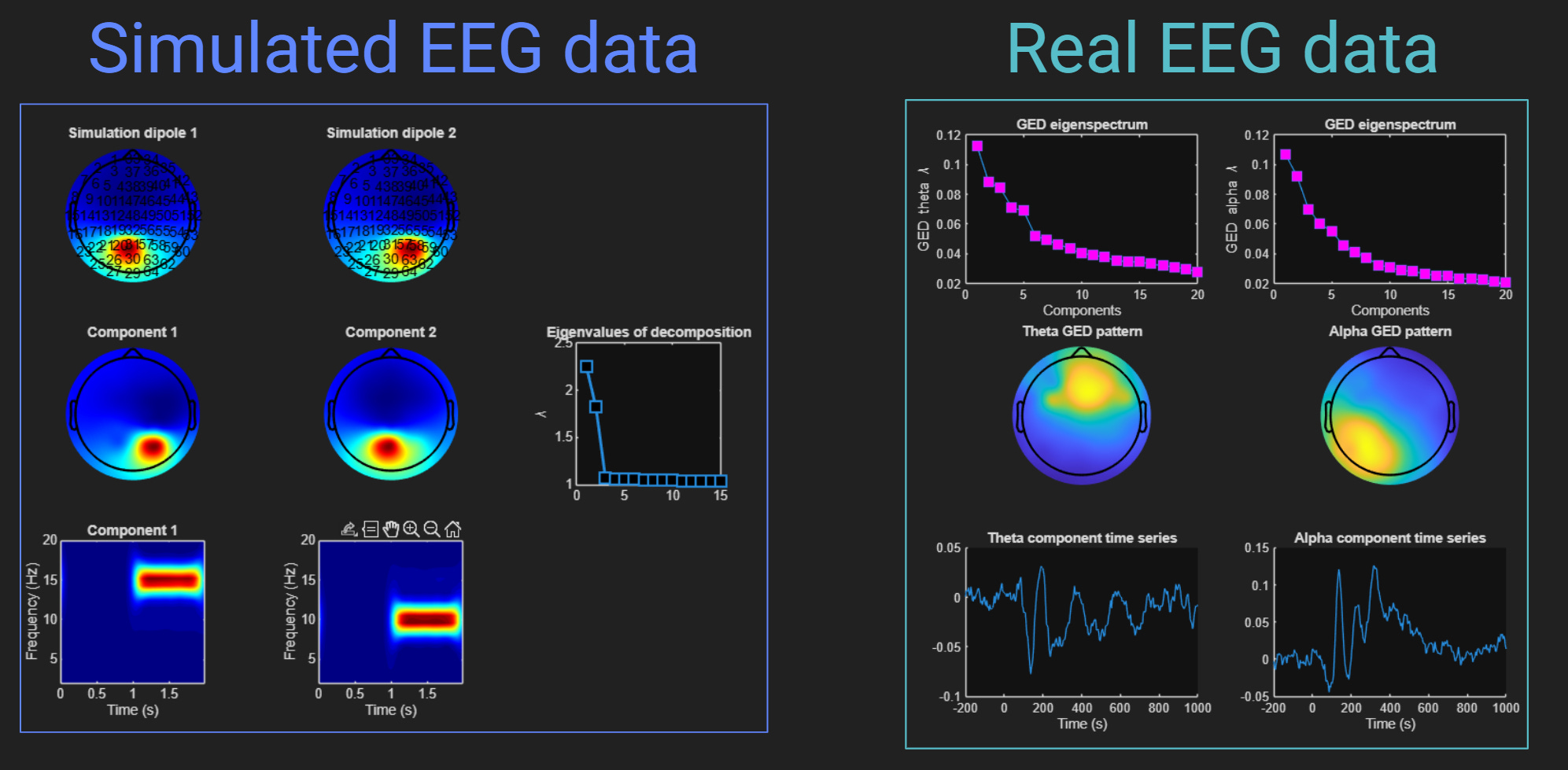
Actually, these are only two of the three deliverables. There is a third figure that you’ll create, but it’s very exciting and I don’t want to spoil the fun.
Both figures above show the result of applying a statistical source-separation method called GED to isolate two components that overlap in time and space, and are separable through a generalized eigendecomposition of two covariance matrices.
Intro to Post 2: Sources, mass-univariate vs. multivariate source analysis
In this first video, I will briefly review a few concepts that I discussed in the beginning on Post 1. I will also motivate multivariate (as opposed to mass-univariate) analyses from both statistical and conceptual perspectives.
Linear algebra crash course, part 1 (theory)
Note: If you are very comfortable with linear algebra, you can skip the next few lectures, or you can watch at 2x speed to get a quick review.
Linear algebra is the branch of mathematics that focuses on matrices and operations acting upon them. It’s arguably the single most important branch of math for data science, AI, computer graphics, and basically anything that happens on computers.
In fact, I’ve written two textbooks (link and link) and a 35-hour course on linear algebra. So yeah, I think linear algebra is pretty awesome 😎
Anyway, I will briefly introduce linear algebra in two parts. This is a rather quick intro and is more focused on the concepts that are important for the rest of this post, as opposed to a deep-dive into the nuances and proofs.
This first part of the linear algebra crash course introduces vectors and matrices, terminology, algebraic and geometric interpretations, and some special matrices like identity, diagonal, and symmetric matrices.
Linear algebra crash course, part 1 (code)
Here you will see the math concepts come alive in MATLAB.
Linear algebra crash course, part 2 (theory)
Here you will learn about covariance matrices and eigendecomposition (a.k.a. eigenvalue decomposition), and some of the special properties of symmetric matrices. There is some math, but I focus more on concepts and visual intuition, as it is relevant for understanding PCA and other multivariate spatial filters.
Linear algebra crash course, part 2 (code)
You’ll create and visualize covariance matrices in simulated and in real data, and you’ll explore eigenvalues and special properties of eigenvectors. You’ll also see what the eigenvectors of random numbers looks like.
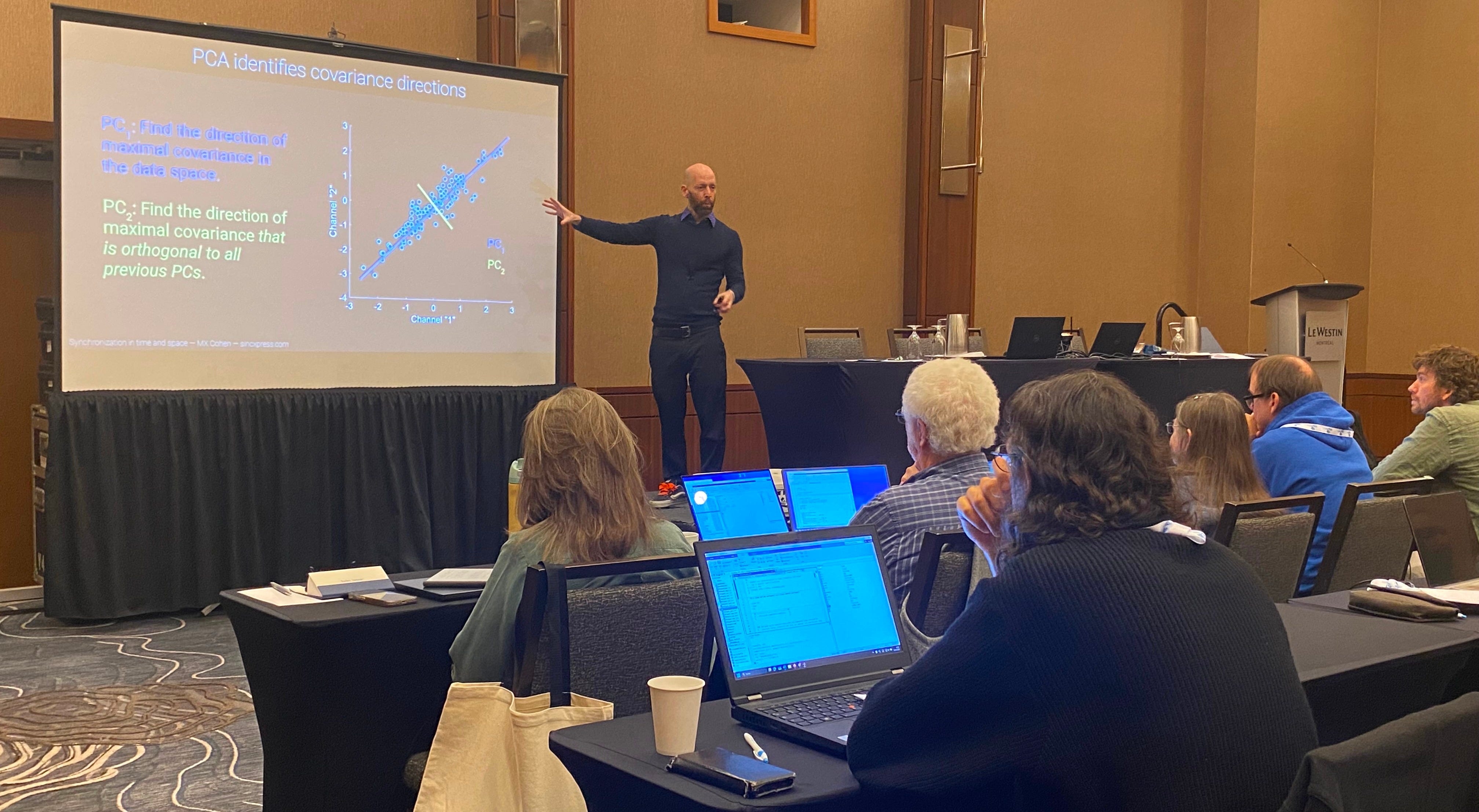
Principal components analysis (theory)
PCA can be introduced and explained in several ways. The approach I’ll take in this lecture is to start with the goal: Find a linear weighted combination of data channels that maximizes the variance of that weighted combination. From that goal, we write an optimization equation, simplify using linear algebra, and discover that the solution to PCA is an eigendecomposition of the data covariance matrix. It’s a beautiful finding 🥰.
This lecture is the most math-intensive in this 2-post series, but I explain the concepts and interpretations, so you’ll be able to understand it even if you’re new to linear algebra.
Principal components analysis (code)
There are two goals of this code file and video.
Show how PCA is implemented in MATLAB — not by calling the
pca()function (although I’ll also show that) but by working through the algorithm step-by-step, starting from mean-centering the data up to calculating the component time series and visualizations.Show the eigenspectrum (aka “scree plot”) of random noise that is normally distributed and non-normally distributed. You might be surprised at the results!
By the end of this video, you will know how to implement a PCA on multichannel data. There’s no EEG data in this video — I want to focus on the code implementations, and I’ll show simulated and real EEG data later.
Generalized eigendecomposition (GED) (theory)
I will begin this lecture by highlighting three limitations of PCA for data analysis. To be clear: these are not problems with PCA; they are limitations of using PCA for source separation in neuroscience data.
Then I will introduce GED as a modification of PCA that is customized for hypothesis-testing. And I will discuss a few key differences between GED and PCA, including that GED vectors are not orthogonal, which is a huge advantage for source separation in mixed-sources data.
Generalized eigendecomposition (code)
Here I will demonstrate how to implement GED in MATLAB code using simple toy example datasets.
GED demos in simulated data (code)
This module involves simulated data to evaluate the accuracy of GED source separation where the ground truth is known (demos in real data are in the next module). There are two demos here:
GED can separate spatially overlapping sources. You’ll simulate data in nearby dipoles that have overlapping topographical projections, and find that GED can separate the sources. This is an interesting follow-up to the inability of the Laplacian to separate these sources.
Compare GED, PCA, and ICA on simulated data. The simulated data will be very simple — just one “signal” dipole and the rest noise — and you’ll run three decompositions on the same dataset. Comparing the results is very enlightening.
GED demos in real data (code)
There’s no substitute for real data! I’ll show three demos in this video:
PCA and GED on broadband data, comparing the pre-trial to trial-related periods.
GED on theta (6 Hz) and alpha (10 Hz) activity. I will also discuss in more detail the versatility of using GED spatial filters in terms of differences between how the filters are created, vs. how they can be applied.
Time-frequency phase synchronization between the components identified in the previous demo. This will tie together everything you learned in the previous and this post.
How to learn more
These two posts are a great way to get started with advanced EEG analysis. If you want to master the topics well enough to apply them confidently to your own data, I recommend the following:
Neural signal processing course
Multivariate signal processing course (including PCA and GED)
Another moment for shameless self-promotion
I hope you enjoyed these two posts! I work hard to make educational material like this. How do I have the time to do it? Well, last month some very kind people supported me by enrolling in my online courses, buying my books, or becoming a paid subscriber here on Substack. If you would like to support me so that I can continue making material like this in the future, please consider doing the same 😊