
EEG synchronization workshop part 1: bivariate phase synchronization
Learn neuroscience EEG signal processing and brain connectivity analyses

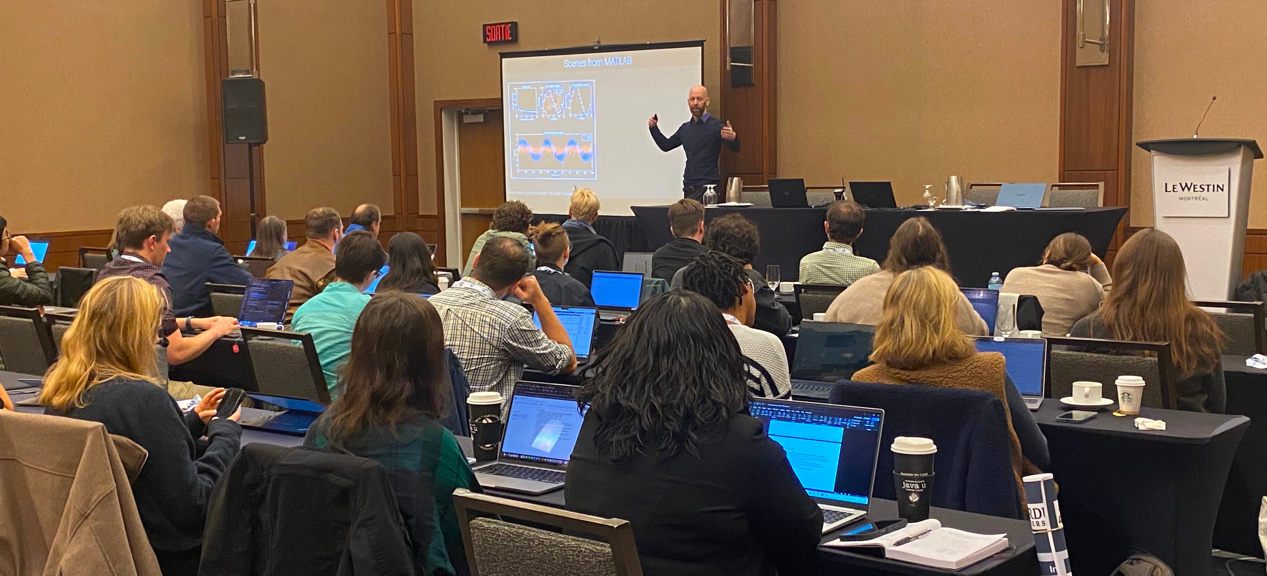
In October 2025, I gave an in-person two-day workshop at the SPR conference in Montreal. 50 people attended and more were on the waitlist. I didn’t want a waitlist — anyone who is self-motivated to learn should have the opportunity to learn — but there were restrictions on the room capacity.
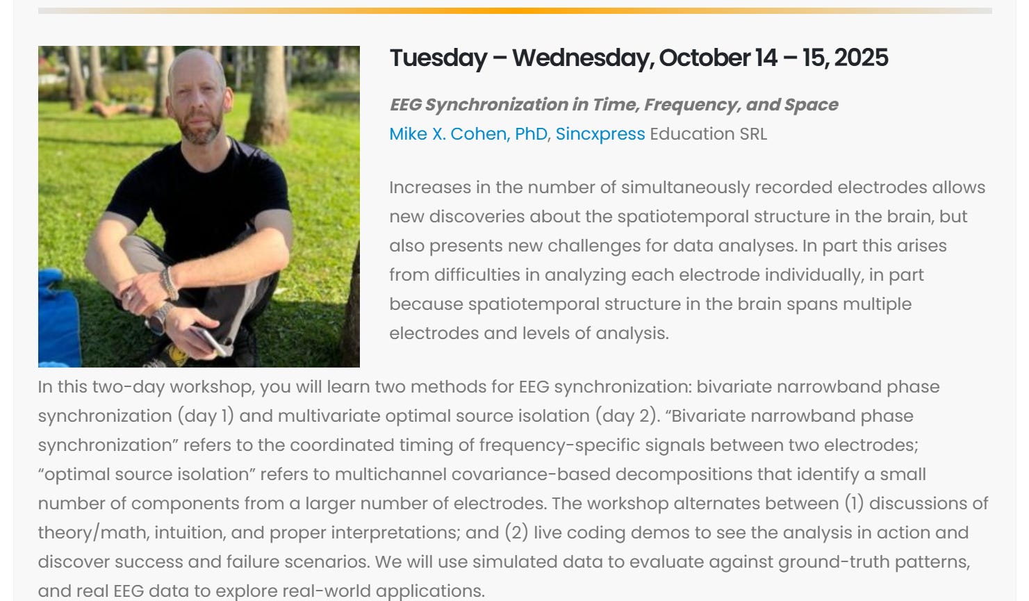
The workshop went well: attendees were positive and gave good feedback, and I felt good about it. I decided to create this two-post Substack text+video series for the people who wanted to be there but couldn’t be, and for the attendees to review and strengthen what they learned.
So here we are :)
Prerequisites and organization of this post
By the end of the two-post series, you will have knowledge and code that will catapult your advanced EEG analysis journey, as well as that buzzing feeling of learning something new and understanding something complicated.
(Here’s the link to part 2.)
Prerequisites: Some experience with EEG and basic MATLAB coding.
Optional additional background material: This YouTube playlist
Organization: There are six modules in this post, each focused on a different topic. They are cumulative, so I recommend going through each module in order. Each module has two parts, a theory part (video lecture with slides, concepts, interpretations, and some math) and a coding part (video walk-through of the code and explanation of the exercises).
How long is this workshop?
How long it takes you to get through this two-post series depends on a number of factors, including your background coding and neural data science familiarity, and on how deeply you want to engage with the material.
If you are just curious to learn about the methods without applying them, then you don’t need to download the code, and you can just watch the videos (perhaps even at 1.25x speed if you’re comfortable with English).
If you want to follow along with the code and do the coding exercises, then each section might take 30-60 minutes. If you do 1-2 sections per day, then the two-post series make you 1-2 weeks.
To be honest: If you really want to master these analyses and publish papers using the methods, then this post series is enough to give you a firm foundation, but there are more nuances and details (e.g., trouble-shooting problems, inferential statistics) that I cover in longer courses. I’ll provide links to specific resources at the end of the next post.
Getting the code and data
Each section has its own code file. You can get all of the code files from my GitHub repo. You can clone the repo if you’re comfortable with git, or just download all the files in one zip. You don’t need to register or login.
Deliverables from this post
By the end of this post, you will create the following figures in MATLAB. What do those figures mean and how do you create them? You have to watch the videos in this post to find out :P
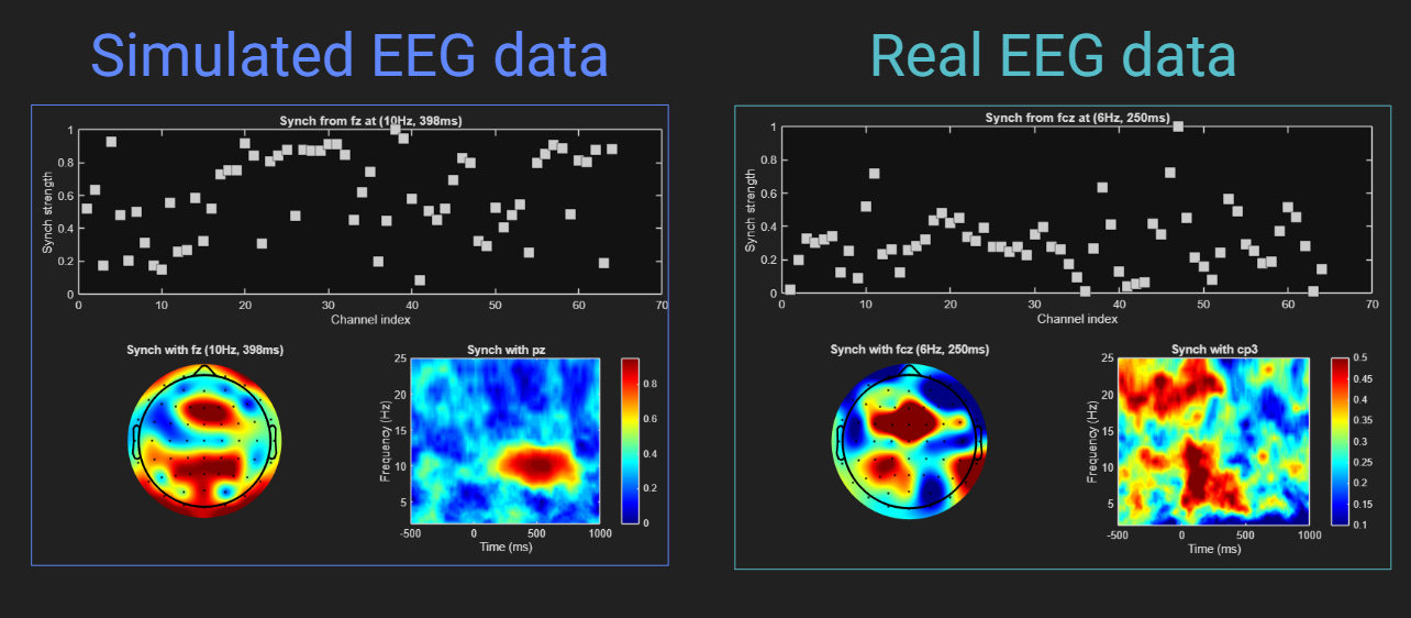
Briefly, the plots show phase synchronization (a measure of brain connectivity) from one “seed” electrode to all other electrodes, over time and frequency. The analysis produces a 3D matrix of synchronization (space, time, frequency), and the plots above show different ways of slicing that matrix. The left panel shows results from simulated data while the right panel shows results from real EEG data. The simulation is used to explore and validate the analysis methods; it’s not meant to be a reproduction of the real data (though you could do that if you want!).
Neuroscience is source separation
This lecture is the intro to the two-day workshop. I argue that all neuroscience research can be described as “source separation.” What does that mean? What’s a “source” and why do sources need to be separated?
The word “source” in neuroscience has multiple equally valid interpretations, including cognitive sources (memory vs. action planning), anatomical sources (hippocampus vs. amygdala), neuron-level sources (pyramidals vs. various interneuron types), circuit-level course (small circuits like a cortical column), spectral sources (theta vs. alpha oscillations), statistical sources (e.g., identified via independent components analysis), and so on. But all interpretations of “source” lead to the same conclusion: Many distinct sources are simultaneously active, and overlap in time, frequency, and space. That’s why they need to be separated.
And how are sources separated? Well, that depends on which definition of “source” you’re focused on: some sources can be separated by experiment design, some by space-based imaging — but most sources are separated by filtering.
Spectral analysis and FFT (theory)
Electrical activity in the brain is strongly rhythmic, and those rhythms modulate brain function from the micro-scale (ion channel dynamics and spike timing) to the macro-scale (perception and consciousness).
Rhythmic activity is present at multiple speeds simultaneously, and are mixed together in the time domain. Spectral analysis is a way to separate those distinct but overlapping sources, and is usually implemented via the Fourier transform. In this lecture, I give a high-level intro to the Fourier transform and how to interpret an EEG power spectrum.
If you want a deeper and more detailed understanding of the Fourier transform, you can consider taking my 7-hour self-paced course.
Spectral analysis and FFT (code)
The video below is a walk-through of the code that implements the concepts I introduced in the previous lecture. I will also introduce the exercises in the code files.
Time-frequency analysis (theory)
Spectral analysis is great, but it’s only really interpretable for stationary signals, meaning that the characteristics of the signals are the same over time.
But the brain is non-stationary. Like, really super duper a lot non-stationary. Brain activity is highly dynamic over time, and so a spectral analysis is a great way to start looking at brain signals, but what you really want is to see how the spectral characteristics change over time.
Enter the time-frequency analysis :)
A time-frequency analysis performs source separation in two dimensions simultaneously: time and frequency (duh…). There are several methods of doing a time-frequency analysis; in this lecture I’ll focus on one method (Gaussian filter-Hilbert). If you really want to learn the details of time-frequency analyses, you can check out my ANTS book and online course. (Note: Gaussian filter-Hilbert is nearly identical to complex Morlet wavelet convolution; I simplified the analysis for this workshop.)
Time-frequency analysis (code)
Now to see time-frequency analysis in action! The goal of this code demo is to produce a time-frequency power plot, step-by-step.
Simulating EEG data (theory)
Broadly speaking, there are two reasons to simulate data in neuroscience:
Computational neuroscience, in which the goal is to test hypotheses about neural dynamics by simulating data with biophysical or morphological constraints.
Analysis methods evaluations, in which the goal is to simulate data that is not biophysically realistic but instead is used to learn about and evaluate data analysis methods.
The first reason is an entire branch of neuroscience, but the focus here is the second reason. Simulating EEG data is a fantastic way to learn about data analysis methods, because simulated data provide ground-truth patterns to compare the results against, and allow you to specify and systematically manipulate signal and noise characteristics.
The goal of this lecture is to explain the concept of simulating EEG data, and to provide more discussion about the pros and cons of using simulated vs. real data in neuroscience education.
Simulating EEG data (code)
Now it’s time to see the simulation in action! I will show how to simulate time series data in the brain, and how to project it out to simulated EEG electrodes.
Synchronization in simulated data (theory)
The title of this workshop includes the word “synchronization,” but I haven’t yet said anything about synchronization. It’s all been necessary background so far.
But you are now smarter than you were at the outset of this post, and so you are now ready to learn about synchronization 🤓. The goal of this video is to present the key concepts, intuitions, and math of phase synchronization.
I will also discuss why synchronization analyses are challenging in real neuroscience data analysis. It’s not because of the math — phase synchronization is actually fairly intuitive — but because of small effects sizes (the brain requires weak connectivity), noisy data, and risk of artifacts. But don’t be dissuaded: synchronization analyses can be fun and insightful. They just need to be done carefully.
Synchronization in simulated data (code)
And now to see how the theory and math are implemented in code. I’ll start with a very simple example of two oscillating signals, and then move on to simulated EEG data. You will observe a confound in electrophysiological synchronization analyses called “volume conduction,” which produces spurious connectivity. That will also be a nice segue into the next lecture on minimizing the risk of volume conduction artifacts through spatial filtering (surface Laplacian).
Laplacian spatial filter (theory)
The Laplacian operator is from mathematical physics and is used to study gradients and flow in heat dissipation among other applications. We use the scalp Laplacian in EEG as a spatial filter that attenuates low spatial frequency topographical components, which are driven by volume conduction. Therefore, the Laplacian spatial filter is necessary for electrode-level phase synchronization.
Laplacian spatial filter (code)
The code in this demo is fairly simple, but the interpretations and conclusions are striking and important. You’ll see the impact of the Laplacian on simulated and real EEG data.
EEG synchronization demos in simulated and in real data
Now to tie together the entire workshop so far! You will integrate the Fourier transform, time-frequency analysis, phase synchronization, and real and simulated data. You’ll also learn about the challenges of multidimensional data visualization, and how to slice the data tensors in different ways to understand brain dynamics.
End of post 1
You are reading this either because you finished going through the post, or because you are curious to see how it ends. Either way: congrats! (although I reserve the bigger congrats for the first group)
Post 2 corresponds to the second day of the workshop, and introduces statistical multi-channel source separation techniques. It’s a different manifestation of brain synchronization, and it also provides another way to examine phase synchronization. You’ll also learn about linear algebra, including matrix multiplication and eigenvalue decomposition.
A moment for shameless self-promotion
Creating posts and videos like this isn’t (only) my hobby; it’s my job. I am a freelance educator. I really enjoy my job (like, really super-duper a lot), but I cannot do it for free. If you’d like to help support me so I can continue writing textbooks, making online courses, and writing these Substack posts, please consider enrolling in my online courses, buying my books, or becoming a paid subscriber here on Substack.
Please also share links to my work with your friends, colleagues, arch-nemesis from high-school, and that one person who you want to befriend but you’re both just slightly too socially awkward to initiate the friendship. Yeah, we all know someone like that.
Hi Mike, thank you for the materials and the workshop at SPR - I learned A LOT! I will be sure to recommend your teaching materials to others. Take care!