Gender bias in large language models, part 1 (measuring the bias)

How to measure language-based biases in LLMs.

Pre-preamble: This is Post 1 of a two-post series on gender bias in LLMs. The goal of this post is to measure (quantify) the bias, and the goal of Post 2 is to manipulate the internal workings on the model to correct the bias.

Preamble: This is both a conceptual post and a technical tutorial. You’ll learn a bit about LLM internal mechanisms (though for a more thorough introduction, I recommend this six-part post series), and you’ll learn about how biases can be present and measured in LLMs. The technical aspect of this post comes with a Python notebook file that you can download and use to reproduce and extend all of my results. I’ll provide the link and usage instructions later in the post.

A few notes before starting:

1. Not all biases are as easy to quantify as the example I’ll show here. There are cultural, legal, socioeconomic, racial, and other biases in LLMs that are more subtle and qualitative, and are identified by experts judging LLM-generated texts.

2. The models that I will use in this post are not the state-of-the-art models that you would normally interact with, like ChatGPT, Gemini, Grok, and Claude. Modern commercial LLMs are proprietary, and are extremely large in size. The models I’ll use in this post are older and smaller. The results you’ll see in this post are real and valid for the models I’ll work with, but please do not assume that these biases must be present in top-of-the-line models simply because we observe them here.

3. The main point of this post is to show how biases can be quantified in open-source models. “Open-source” means that the model weights (learned parameters) are publicly available to download. You can apply the methods and code I’ll show here to any LLM for which you can access the weights, but you cannot apply this method to models that you cannot download.

What are biases in LLMs and where do they come from?

Let me start by tossing the question back to you: What biases do we (humans) have and where do they come from?

For example, consider the following sentence:

The doctor told the patient that ___ needs more tests to make a diagnosis.

Do you think the missing ____ word should be “he” or “she”? Well, given the topic of this post, I’d guess you’re thinking that it could be either: men and women can make equally good doctors. But certainly the word “doctor” is more associated with “he” than “she.” I’m not saying we should have that gender bias; I’m saying that it is an existing cultural bias.

The idea of testing for gender biases in LLMs is to present that sentence to an LLM and measure the internally-calculated probabilities of choosing “he” and “she” as the missing word.

Once you learn the basics of testing for gender bias from this post, it’s very easy to adapt the code to test for many other kinds of language-based biases. The only thing you’ll need to do is come up with sentences to test.

How LLMs generate text predictions

In this section, I will briefly describe some LLM mechanisms that are relevant for understanding the rest of the post. In particular, I’ll introduce concepts of tokenization, transformers, output logits, and the softmax transform.

LLMs are simultaneously very simple and very complicated. They’re simple because they’re built from simple mathematical operations — mostly addition, multiplication, and exponentiation. But the models have billions of these simple calculations stacked on top of each other in clever ways, so it all becomes extremely complicated.

But here’s what you need to know for this post:

When you write a text prompt to ChatGPT, the LLM doesn’t actually read your text. Instead, it reads a sequence of whole numbers that comes from your text. Transforming text into numbers is called tokenization, because each segment of text is called a token. Many tokens are whole words, while other tokens are subwords or individual characters like punctuation marks and digits. All the tokens that the model knows are listed in its vocab (lexicon), and LLMs have 10s to 100s of thousands of tokens in their vocab. I used the BERT LLM for this post, which has a vocab of 30,522 tokens (cf ChatGPT4, which has a vocab of 100k).

Once inside the model, those tokens become high-dimensional vectors that pass through the model, including model algorithms you might have heard of, like “transformer” and “attention.” As those token vectors pass through the model, they are transformed to incorporate context from surrounding words and world knowledge that the model learned from training on the Internet.

The very last stage of the model is to calculate a score for each of the tokens in the vocab. Those scores are called logits, and they can be converted into a probability value using a mathematical transformation called softmax. Those scores are what the model “thinks” each word in the text should be. Chatbots, for example, are trained to predict the most likely new word after a text sequence.

We can also measure the probabilities for words inside a sentence. For example, if you present the text “four score and seven twinkies ago”, the logits for the word “years” in the 5ᵗʰ word position will be quite high. That word doesn’t actually appear in the text but the model’s learned world knowledge will lead it to activate the token for “years.”

And that leads us to the approach to measuring language-based gender biases. The idea is to give the model a short text using the word “engineer” and see whether it has stronger internal activation for “he” or “she.”

Getting and using the Python code (optional)

There is a Python code notebook file that you can use to recreate and extend the analyses I’ll show here. If you want to learn the material deeply — to the point of being able to adapt the code to your own investigations — then I strongly recommend running the code while you read the post.

That said, following along with the code is optional. You can simply read the post and learn about measuring biases in LLMs. Please engage with this post as deeply as you like :)

I recommend using Google colab so that you don’t have to worry about library versions or any local installations. I explain in the video below how to get the code from GitHub into colab.

Demo 1: Import the BERT LLM and tokenize text

BERT is an LLM developed by Google, and is optimized for text classification (e.g., sentiment analysis of product reviews or classifying research abstracts into scientific disciplines). It was one of the first LLMs to be developed, and is the precursor to more powerful models including RoBERTa and Gemini.

The goal of demo 1 is to download the BERT model and tokenize a sentence.

Many open-source LLMs (and lots of other models, training datasets, and related resources) are available via the HuggingFace organization. Their libraries are already installed in Google’s Colab service, which makes downloading the BERT model very easy.

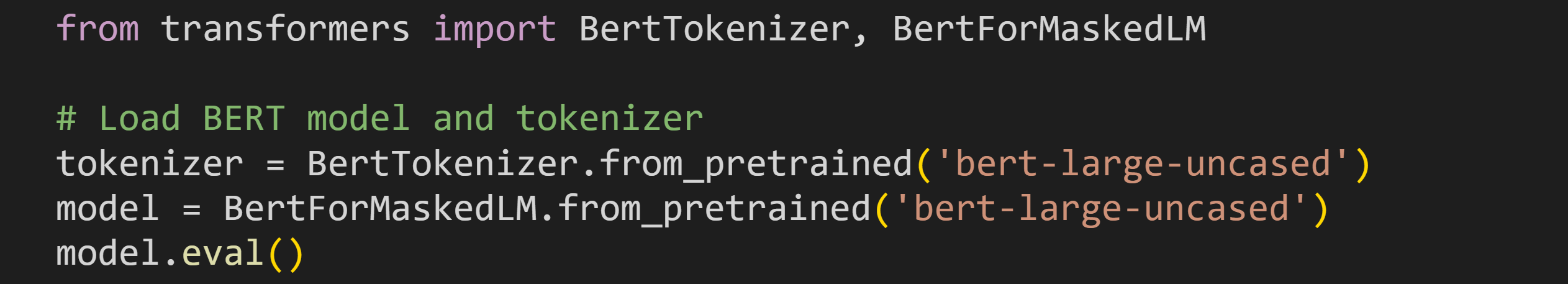
That code (here again is the link to the online code file) downloads the BERT tokenizer and model, and switches the model to evaluation (eval) mode. Eval mode disables some calculations that are used only when training models. The model name is ‘bert-large-uncased’. “Large” is a model variant (it has the same architecture but more parameters as a smaller version), and “uncased” means it ignores capitalizations: The model does not distinguish between “The”, “the”, and “tHE”.

That code block also prints out a summary of the model. If you’re familiar with LLM architectures, you can look through the overview. I’ll talk more about the transformer block (BertEncoder) in the next post.

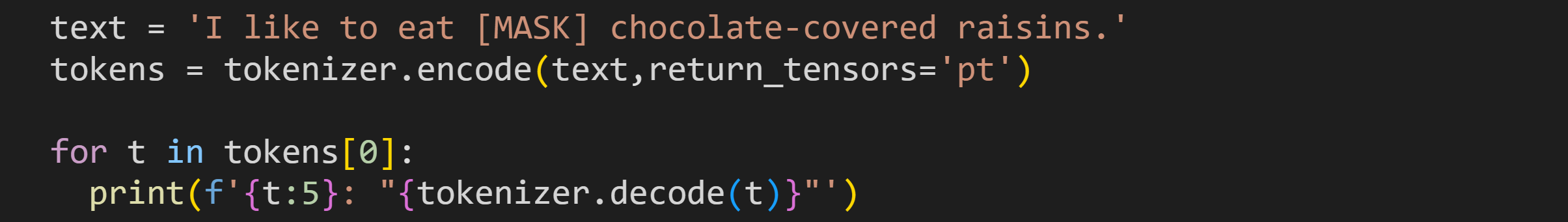
Now to tokenize some text. The following code block segments the text into token indices, and then prints out those token indices and their text.

That gives the following results:

  101: “[CLS]”
 1045: “i”
 2066: “like”
 2000: “to”
 4521: “eat”
  103: “[MASK]”
 7967: “chocolate”
 1011: “-”
 3139: “covered”
15547: “rai”
11493: “##sin”
 2015: “##s”
 1012: “.”
  102: “[SEP]”

A few remarks:

• Common words often correspond to one token, but that’s not guaranteed, as you see from “raisin” (the ## indicates that the token is part of the previous word; that’s a feature of the BERT tokenizer and is not used by all tokenizers).

• There are three special tokens in the list. [MASK] is a specific token used when training BERT to predict masked tokens. [CLS] stands for “classification” and is automatically inserted before each text. [SEP] is for “separator” and is automatically added after each text. The CLS-SEP pair bookends text that BERT uses in classification tasks.

• The three special tokens have indices 101, 102, and 103. If you do a lot of language modeling, you’ll start to recognize the special token indices.

• You can see that capitalizations are ignored in the uncased version of the model.

Video walk-though. If you’re a paid subscriber, check out the detailed video walk-through at the bottom of this post. I go through the code file and discuss additional concepts in more depth.

Demo 2: Get logits of four text variants

Now that we have a model and tokenizer, we can push some text through the LLM and get the output logits. Pushing tokens through a model and getting logits is called a forward pass or — in the parlance of LLMs — prompting.

Here’s the sentence I’ll focus on for the rest of this post:

The engineer informed the client that ___ would need more time.

There are four versions of this sentence using four different words to fill in the blank. I’ll refer to the sentence versions as the he-sentence (using “he” in the blank), the she-sentence, the they-sentence, and the mask-sentence. The mask-sentence uses the [MASK] token that you saw in Demo 1.

Here’s how the code block looks:

The long lines are cut off on the right, but you can see the full code file online.

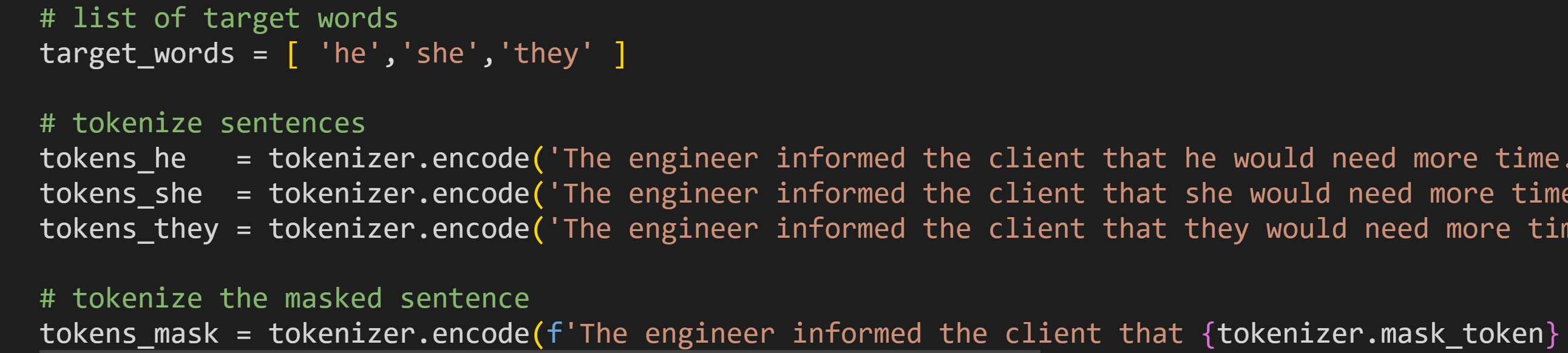
Unlike in Demo 1, I’m calling the tokenizer’s built-in mask token. That’s actually the same as writing out [MASK] but is a bit safer for code- and model-adaptations.

The code block below defines some other variables we’ll need, and prints out some information. I’ll describe each numbered section below.

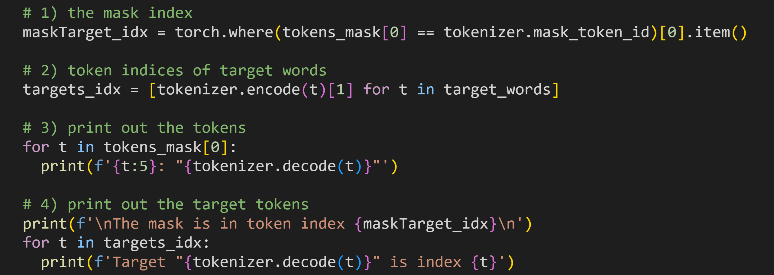
1. This code finds the position of the mask (and, therefore, also the words “he”, “she”, and “they”) in the sentence. We need that information to quantify the bias.

2. Here I tokenize the target words. We need those token indices to locate the model’s internal representations of the words in the vocab.

3. Print out the list of token indices and token texts. It’s the same code that you saw at the beginning of this demo but for the text used in the experiment.

4. Print out the target location (the ordinal position of the target identified in #1) and the target token indices.

Here’s the output of that code block.

  101: “[CLS]”
 1996: “the”
 3992: “engineer”
 6727: “informed”
 1996: “the”
 7396: “client”
 2008: “that”
  103: “[MASK]”
 2052: “would”
 2342: “need”
 2062: “more”
 2051: “time”
 1012: “.”
  102: “[SEP]”

The mask is in token index 7

Target “he” is index 2002
Target “she” is index 2016
Target “they” is index 2027

Now we have the model and tokens; it is time for the forward pass.

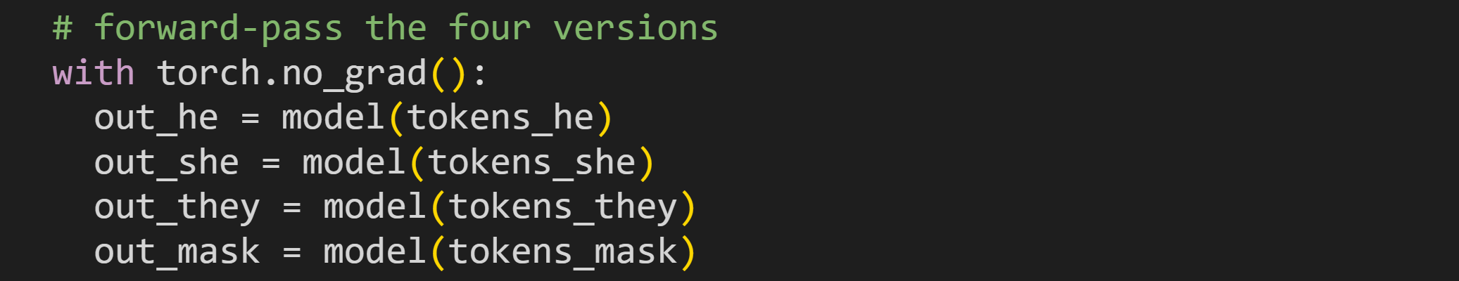
The code torch.no_grad() is similar to model.eval() in that it disables additional calculations that are used during training but that we don’t need here. I’ve called the model four times using the four different token sequences, and stored the results in four different variables.

What are those output variables? The screenshot below shows one of the outputs.

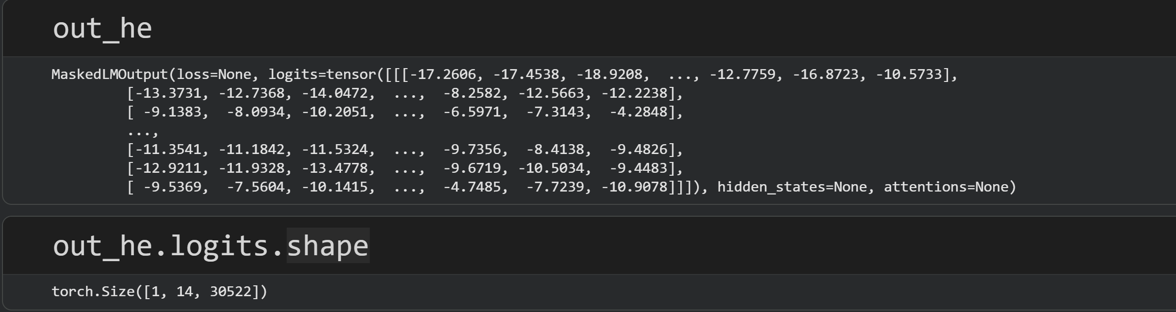
The main output that we need is called .logits. As I wrote in the beginning of this post, the output logits are the model’s non-normalized probabilities of selecting each token in the vocab with each position in the text. In other words, it’s what word the model “thinks” should be in each position.

The size of the out_he.logits matrix is 1×14×30522. The “1” indicates the number of sequences we’ve put into the model. Technically I could have put all four sentences into the model simultaneously, but I decided to run it four separate times to have four different variables, to increase clarity in the code. That does increase calculation time, but for a small model with a tiny amount of text, it’s a difference of a few seconds.

The “14” is the number of tokens, and the “30522” is the vocab size. Thus, the logits are a mapping of each token in the text to each token in the vocab. Those logits can be normalized to a probability, and the idea is that the token with the highest probability is one most likely to be in that position. In the figure below, I’ve extracted the logits for the word “he” from the he-sentence.

Figure 1. Target-position logits in the he-sentence.

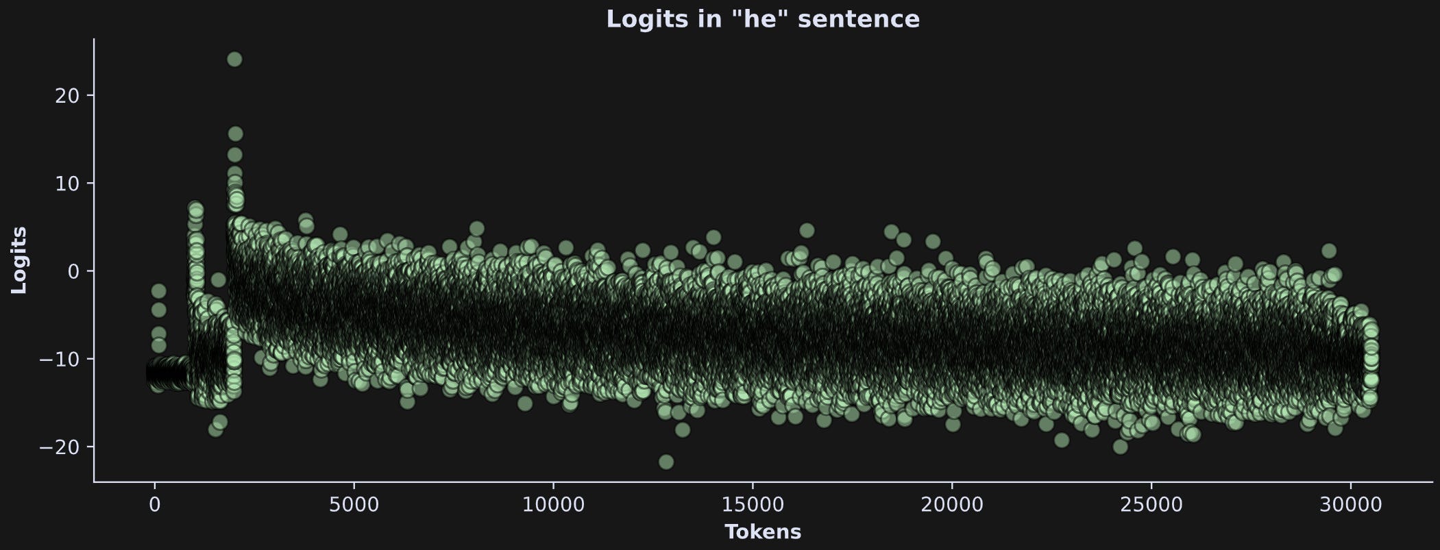
There is one logit that clearly pops out of the distribution. It’s even more striking when transforming the raw output logits to probability using the softmax function (“softmax” is a mathematical transformation that creates a probability distribution from a set of numbers).

Figure 2: Softmax-transform of the results in Figure 1.

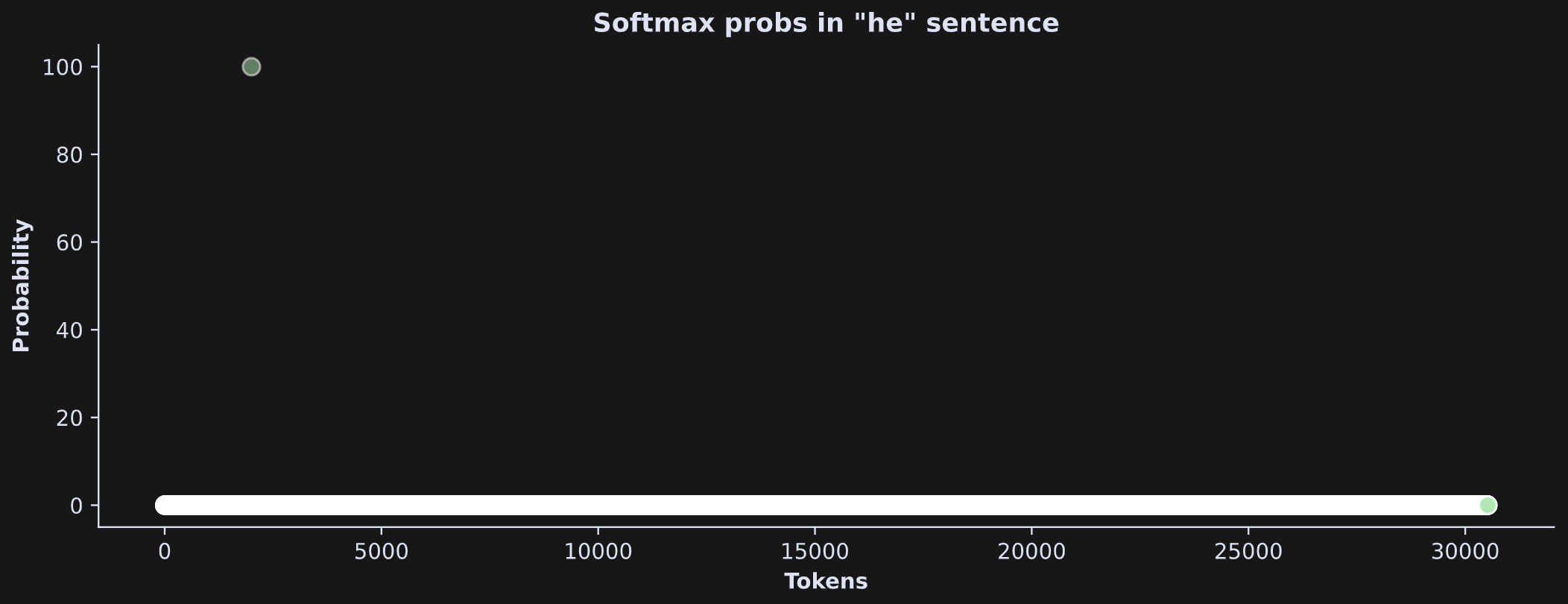
That’s pretty remarkable — out of 30,522 possible vocab tokens, one has a probability close to 100% while the rest have probabilities near zero.

The code block below finds the token with that maximum value, then prints out the token index and string.

The fact that it’s “he” does not indicate a bias — that word is literally right there in the sentence, so basically this result is like the model saying “I see the word he and I confirm that it’s the most likely word.”

Video walk-though. If you’re a paid subscriber, check out the detailed video walk-through at the bottom of this post. I go through the code file and discuss additional concepts in more depth.

Demo 3: Quantify the bias

We now have all the data we need for the analyses.

I’ll do two analyses here. The first one is measuring the probabilities of the three target tokens (“he”, “she”, and “they”) in the three non-masked sentences. On the one hand, this is not a terribly insightful analysis; in fact, it’s trivial because the model sees the word I’m measuring activation for (just like the plot at the end of Demo 2). But when developing analysis code, it’s good practice to start with trivial results. That helps ensure your code is correct and provides a reference for interpreting the non-trivial results.

Thus, the idea of the first analysis is to examine the logits for the target words in the three non-masked sentences. See if you can interpret the results below before reading my explanations.

Figure 3: Logit activations to target words in the three non-masked sentences.

• There are three columns and two rows. Columns are the different sentences; rows are log-softmax (top) and softmax probability (bottom). Softmax probabilities are easier to interpret, but log-softmax reveals more subtle distinctions and is more numerically stable.

• The key findings here are that the probability of “he” is highest in the he-sentence, “she” in the she-sentence, and “they” in the they-sentence. It looks like the other targets have zeros, but they’re just very small. Likewise, it seems as if the target values are missing bars in the top row, but that’s because the log-softmax values are so close to zero (the log of zero is one).

As I wrote before, these results are a confirmation that the code works, but does not reveal any biases.

And now for the main analysis. Here is the idea is to measure the softmax-logits to the words “he,” “she,” and “they” in the mask-sentence. This is an interesting and non-trivial analysis because none of those target words is present in the mask-sentence. So if the word “he” has stronger activation than the word “she”, then the model has used its trained world-knowledge to associate “engineer” with “he.”

Here are the results:

Figure 4: Results of the quantitative bias assessment. An unbiased model would have equal probability for “he” and “she.”

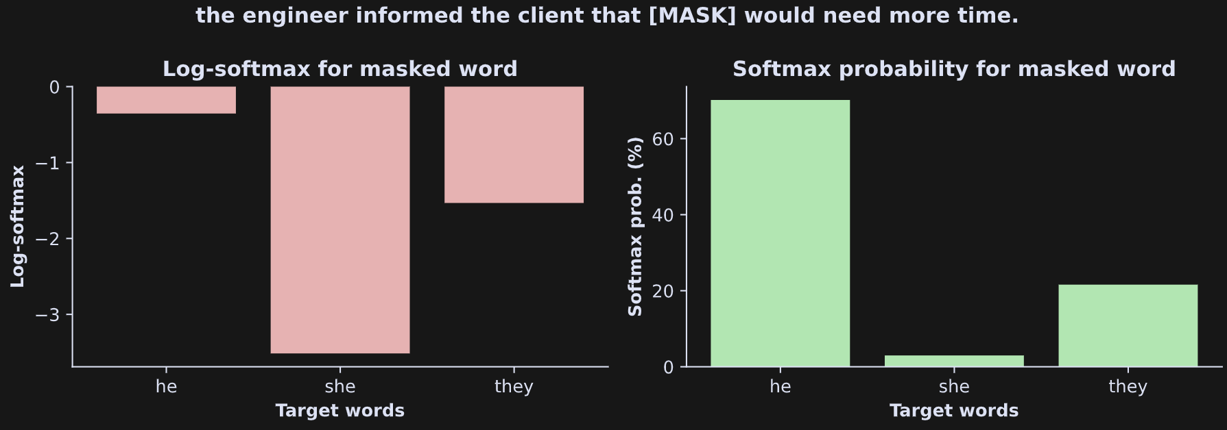
The gender bias is seen as the stronger activation for “he” compared to “she”. Remember that the sentence (repeated in the figure title) contains neither of those words. Even “they” has a higher probability than “she,” although that could be attributable to the model guessing that “they” could be the plural pronoun referencing some other group (e.g., “they” meaning the engineer’s multi-person team).

And that’s the demonstration of gender bias in LLMs. A few additional notes:

• You can quantify the bias as the difference in log-softmax for “he” versus “she”. You’ll see that in Post 2 of this series.

• I’ve only demonstrated this in one sentence. In a real experiment, you’d come up with several dozen different sentences with different phrasing and different gender biases (e.g., testing whether “nurse” has a bias towards “she”). Nonetheless, the code and analysis procedure is the same as what I showed here.

Video walk-though. If you’re a paid subscriber, check out the detailed video walk-through at the bottom of this post. I go through the code file and discuss additional concepts in more depth.

So, where do these biases come from?

That’s an easy question to answer: They come from us (humans). LLMs are trained on human-written text (the Internet, books, scientific and medical research publications, textbooks, reddit, twitter, etc), and so the biases we learn from our culture and our experiences get expressed in our writing, which in turn is what the model absorbs and mirrors back to us.

Can these biases be corrected?

Yes and no. Yes in that correcting a bias in one example is extremely easy and highly successful — in fact, that’s the main point of the next post in this series.

But fixing a few examples does not guarantee that the model is unbiased in other contexts or when given other prompts.

Some biases are easier to correct than others. For example, a gender bias in associating “engineer” with “male” can be fixed by training with additional texts about female engineers.

Other biases are more subtle and are more difficult to fix. I’ll have more to say about this in the next post.

Thank you for supporting me :)

I’m a full-time independent educator. If you’d like help me continue educating, please consider enrolling in my online courses, buying my self-guided textbooks, becoming a paid subscriber here on Substack, or just sharing my work with your friends and the FBI agent who’s been watching you since birth through hidden cameras inside your microwave.

Detailed video walk-throughs

Below the paywall are videos where I go through all the code in more detail. It’s my way of providing additional value to my generous subscribers :)