
LLM breakdown 2/6: Logits and next-token prediction
Learn how language models (including chatbots) generate new text

About this 6-part series
Welcome to Post #2 of this series!
The goal of this series is to demonstrate how LLMs work by analyzing their internal mechanisms (weights and activations) using machine learning.
Part 1 was about tokenization — how text is transformed into integers by chunking groups of characters that often appear together in written language (e.g., “the” is one token). Tokenization is the first step in the journey of text through an LLM.
The final step in the journey through an LLM is the output logits. Those are numbers that the model uses to make predictions about what token should come next.
Therefore, after reading the previous and this post, you will understand the two ends of an LLM, where information goes in (the mouth) and where newly generated text comes out (the… uh, well, I’ll leave that to your imagination).
Use the code! My motto is “you can learn a lot of math with a bit of code.” I encourage you to use the Python notebook that accompanies this post. The code is available on my GitHub. In addition to recreating the key analyses in this post, you can use the code to continue exploring and experimenting.
What are logits and where are they in language models?
The word “logit” has a specific meaning in statistics: It is a number associated with a probability of a binary event occurring (specifically, the logarithm of an odds ratio). But you don’t need to worry about that definition here. The important thing to know for an LLM is that the logits are the final numerical outputs of the model, which are transformed into probabilities of picking a new token.
Remember from the previous post that tokenizers have a vocabulary that contains all of the tokens the model has been trained on. In OpenAI’s GPT2, the vocab contains 50,257 tokens. There is one logit value per token; thus, the final output of an LLM is a vector of 50,257 numbers that is associated with each input token. So if your text has 5 tokens, then the final output of the model will be a matrix of size 5x50257.
Why does each input token get its own vector of output logits? Because the goal of an LLM is to transform each token into a prediction for the next token. For all but the final token, we can match the prediction to the actual next token (in fact, this comparison is how LLMs are trained); and for the final token, this vector of logits is used to generate a new token.

Figure 2 below shows an example of logits (copied from my post about creating text heatmaps). The x-axis has 50k elements, the y-axis shows the logit value, and the token index with the largest logit is highlighted in red.
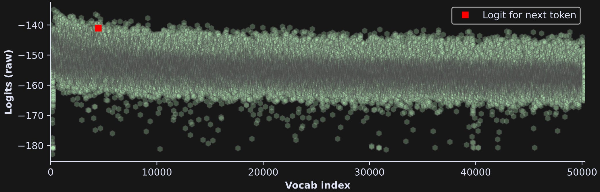
Basically, this plot shows that the model makes a prediction for what the next token should be. An ideal response is for most of the tokens to have relatively small values, and a small number of tokens have relatively large values.
Getting logits from a model
Getting the output logits is very easy in Python. You just need to import a model and input some text. Here’s how to import GPT2 (the “small” version, which has 125M parameters) using the HuggingFace library:
(Friendly reminder that only the essential code lines are printed in the post; fleshed-out and commented code is on my GitHub.)
Now for some tokenized text:
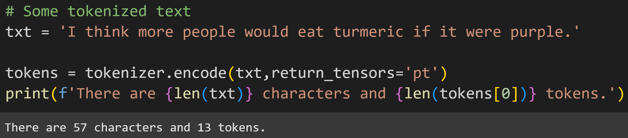
Most of this code should look familiar from the previous post on tokenization. But the second input to the tokenizer (return_tensors=’pt’) is new. The tokenizer’s encode method returns a list of token indices, but the model expects a PyTorch tensor data type. The 'pt' stands for PyTorch.
Now to process the tokens. This is what happens when you press the Enter key in your chatbot window. You will learn much more about the internals of LLMs in later posts, but the idea is that the tokens are transformed into embeddings vectors, then passed through a sequence of transformer blocks that modify those embeddings vectors so that they indicate a prediction about what token should come next.
This step is called a forward-pass or inference, and it looks like this:
model.eval()
with torch.no_grad():
  output = model(tokens)
The key line is output = model(tokens). If you’re new to deep learning and the PyTorch library, then the other lines might look strange. model.eval() is a toggle that switches the model into “evaluation mode,” which means that it switches off calculations that are used during training (e.g., dropout and batch-norm regularizations). The line with torch.no_grad() deactivates the calculations of the gradients and other housekeeping elements of the computational graph that are necessary for training but are not for applications.
Switching off the gradient calculations isn’t necessary here, because the text is so small that we’re not really saving any meaningful computation time. But it’s good to get into the habit of doing a forward pass without the extraneous calculations.
Anyway, the variable output has many attributes that I encourage you to inspect by running dir(output). The only attribute that we care about in this post is the logits:
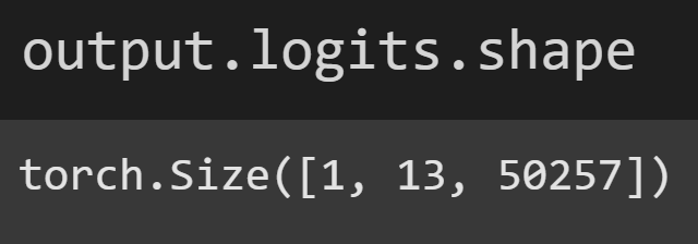
The logits is a 3D tensor — like a stretched-out cuboid. What do those dimensions correspond to? The “1” is for sequence in a batch. LLMs are designed to process multiple text sequences simultaneously. That’s used for training in batches of, e.g., 64 chunks of text. We’re only processing one sentence here, so there is only 1 sequence. (This is also why I indexed tokens[0] in Figure 3.)
The “13” is the number of tokens in the sequence. And the “50257” is the number of tokens in the vocab. Thus, each token in the sentence has an entire vocab’s worth of numbers. Those numbers are the logits, and correspond to what token the model thinks should come next. For example, the 5th token is the word “ would” and its logits look like this:
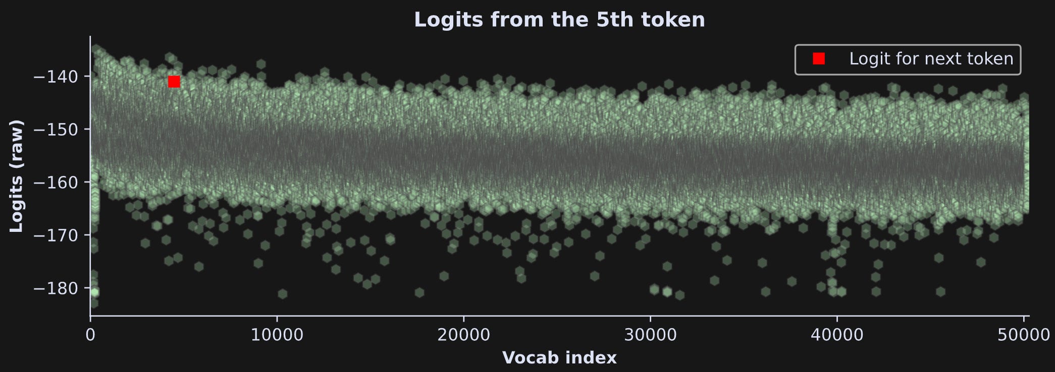
That red square is the logit for the token position for the subsequent word (“ eat”). In theory, that token should be the largest out of all the tokens. It isn’t, which means the model made an incorrect prediction. In fact, the largest logit — the text that the model predicts should be next — is “ be”. That is technically incorrect (the best kind of incorrect), although it is a very sensible prediction: “I think more people would ____”
Anyway, what I want to discuss here is the y-axis. What do those numbers mean and how do they relate to actual predictions of tokens? For several reasons, those numbers are not actually directly interpreted. Instead, we need to convert them into a probability distribution via the softmax transformation.
The softmax function that creates probabilities
Softmax is a way to transform any set of numbers into a probability distribution. What’s a probability distribution? A probability is the chance of something happening or being observed, like “30% chance of rain” or “.00000001% chance of winning the lottery.”
A probability distribution is a set of probabilities that sum to 100% (or to 1 if not scaled up by 100). For example, “30% chance of rain” is not a probability distribution, but if we’d add to the set “70% chance of no-rain” then we’d have a probability distribution.
Another part of the definition of a probability distribution is that all the possibilities in the set need to be mutually exclusive. Consider, for example: “30% chance of rain, 40% chance of snow, 60% chance of no precipitation.” Those numbers sum to 130%, but the summing doesn’t make sense, because it can rain and snow at the same time.
Unlike inclement weather, token selection is mutually exclusive: One token gets selected; it’s not possible to have 13 tokens in the same position at the same time. This means that we can create a probability distribution from logits.
But the “raw” logits are not probability values (obviously: they are negative and, in the example in Figure 5, sum to -7,789,878). Enter softmax.

The softmax function is often indicated using the Greek letter σ (sigma). It is defined as a ratio of each data value divided by the sum over all n data values, after exponentiating those data values. The exponentiation is used because e^x is positive for any value of x (including negative values!). And when you sum together all n data values, you get the sum divided by the sum, which is 1. Thus, it fulfills the definition of a probability distribution.
Softmax is deceptively simple. There are some important nuances to the softmax transformation that are related to the nonlinear properties of e^x. There is also a parameter in the softmax function that I omitted from the formula, called temperature, that affects how much the transform “bends” the raw data. I will have a separate post dedicated to softmax (will be linked when I write the post!), but for now, suffice it to say that the softmax doesn’t just rescale to a probability distribution; it also stretches the distribution so that relatively small values get suppressed while relative larger values pop out of the distribution.
Because the equation for softmax is simple, we should be able to translate it directly into code:

That second line of code should work, but it doesn’t. It produces a vector of nan’s (not a number). There’s nothing wrong with the math or the code, but there are numerical inaccuracies and computer rounding errors that accumulate with a large number of very negative values. The PyTorch function F.softmax has some built-in “softeners” that prevent numerical issues (e.g., adding a small constant to the denominator).
Anyway, here’s what the logits look like before and after softmax’ing:
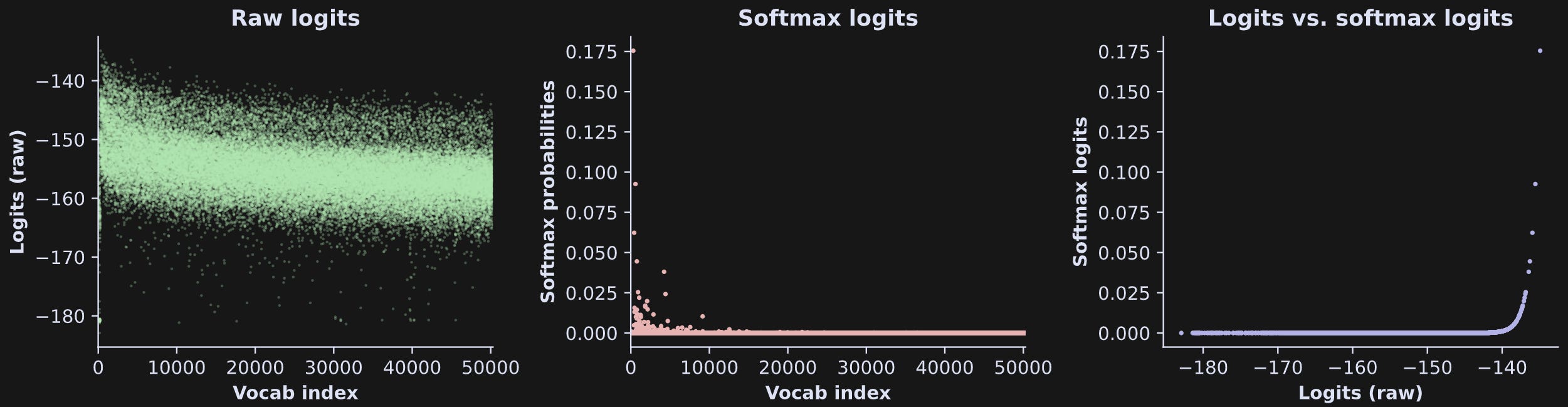
Quite striking, wouldn’t you say? The softmax transformation suppressed most of the token logit distribution while boosting one token (look for the pink dot near the upper-left corner of the center panel).
One more concept I want to introduce before talking about text generation is the log-softmax, which simply involves taking the natural log of the softmax data. The log transform is defined only for positive values and pulls tiny numbers close to zero down towards -∞.
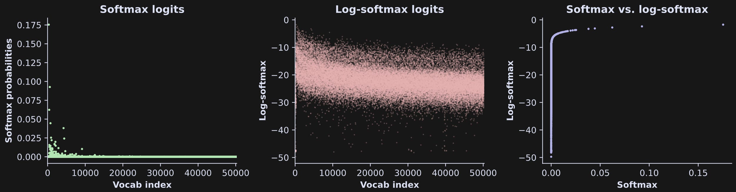
It looks like the log-softmax brought us back to the original raw logit values. It kind of did, because the natural logarithm and natural exponential are inverse functions of each other, although the numerical values are different than the original raw logits.
I won’t use log-softmax for the rest of this post, but it is often used in LLM training and interpretation, so I decided to include it here.
How LLMs generate new text
The distribution of logits for the 5th token is the model’s prediction about the 6th token. When there is a 6th token, we can compare the model’s predictions to the actual token, and models are trained to maximize that prediction accuracy (technically, they’re trained to minimize the inaccuracy).
What happens when there is no 6th token? The logits for the final token in a sequence are used to generate a new token that would follow that sequence.
It works like this: given the text “I like oat milk in my”, what do you predict comes next? Well, you don’t know for sure, but you can use context and world-knowledge to narrow down the list of possibilities to something like “coffee” or “cereal.” The next token is certainly not “)” or “<html>” or 50k other tokens. As you now know, each token in the model’s vocab has a logit value, and the logit value for the final token (“ my”) is the prediction about the next token.
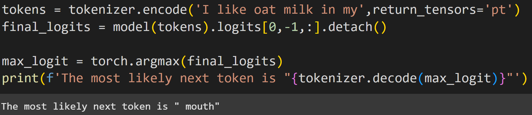
The screenshot above shows that GPT2 predicted that the next token should be “ mouth”. Is that the correct response? There is no text to compare it to, but “I like oat milk in my mouth” is certainly grammatically accurate and contextually sensible (though a bit silly).
Figure 9 below shows all the logits and the token index with the largest logit.
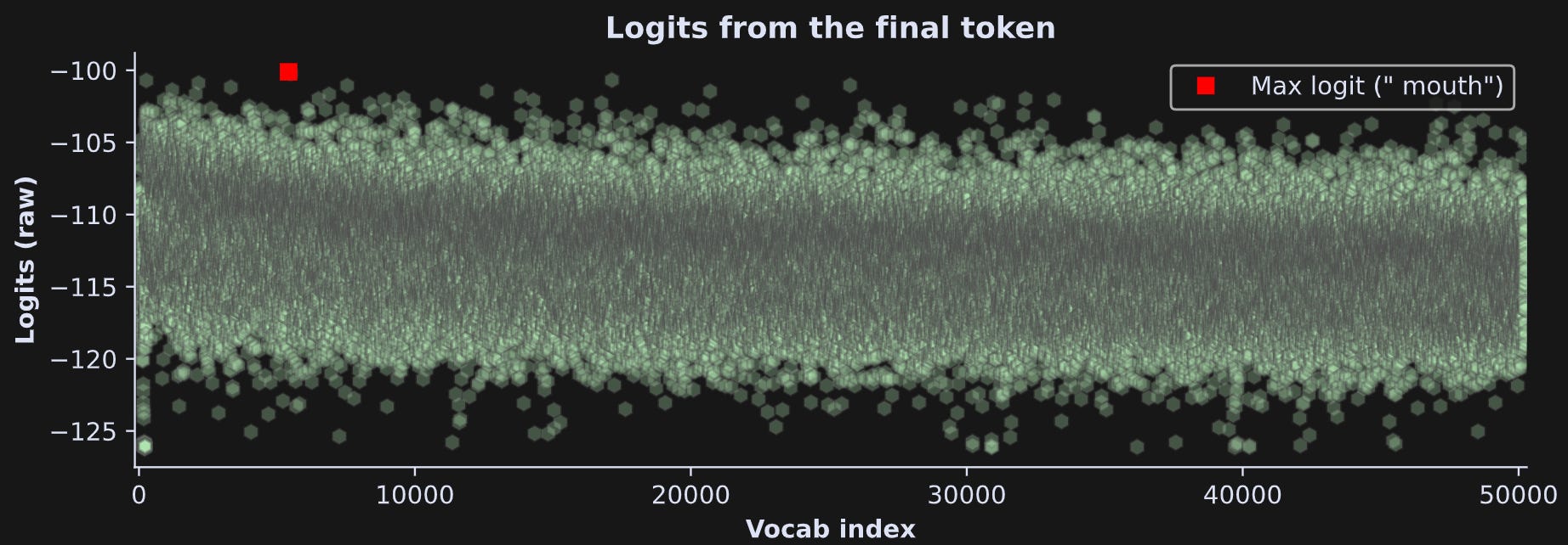
Two remarks:
If we’re just picking the token with the maximum logit, we don’t need to transform the data. Softmax and log-softmax are monotonic transformations, meaning that the sorting is preserved before and after the transformation.
Although the token “ mouth” has numerically the largest logit, it’s not that much bigger than many other tokens. Indeed, it’s not really clear (to my eye at least) purely from visual inspection that that’s the largest. This means that the model calculated several tokens to be roughly comparably likely.
Let’s follow-up on that second point. The screenshot below shows the top-10 tokens.
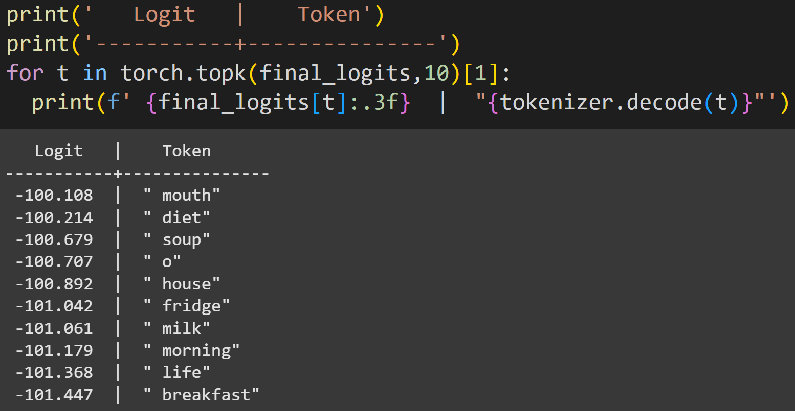
The token for “ mouth” is numerically the largest, but not by much.
Where’s the coffee? If you enjoy hipster coffees or are lactose-intolerant, you might be surprised to see that “coffee” is not in the top-10. Let’s find its position. See if you can understand what the following code block does, before reading my explanation below.
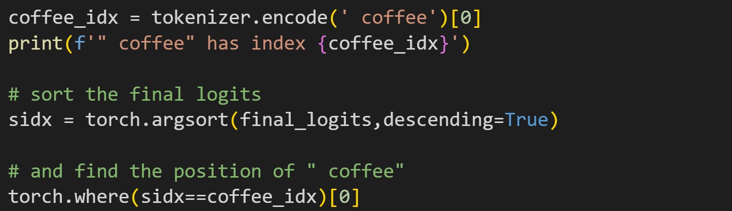
The idea of the code is to sort the logits, then find the position in which the token for coffee appears. The output of torch.where is “12”, meaning that coffee is the 13th highest logit. (btw, try running that code without the preceding space in “coffee”!)
Probabilistic token selection
Should LLMs always pick the token with the largest logit? Not necessarily. Deterministic models are kind of boring — more predictable, but boring. And that’s not how commercial chatbots models work: You can give an identical prompt to ChatGPT 10 times and it will give you 10 different replies. In practice, the model picks a new token to generate based on a few possible methods:
Greedy. That’s what I showed above — take the token with the largest logit.
Top-k. Find the top-k tokens and pick one at random. In Figure 10 above, k=10.
Top-p (aka nucleus sampling). Transform the logits to softmax-probabilities and sort by descending probability. The smallest set of tokens that adds up to p% is taken, the probabilities in that set are re-normalized, and then one token is chosen based on those probabilities. Typical values of p are 90% or 95%.
Multinomial. Choose randomly from all tokens, but each token is selected according to its probability in the softmax-logits. In theory, any token in the dictionary can be selected, but the probabilities of most tokens are exceedingly low.
The figure below shows an example of multinomial selection. I convert the logits to softmax, then use those probability values to select five.
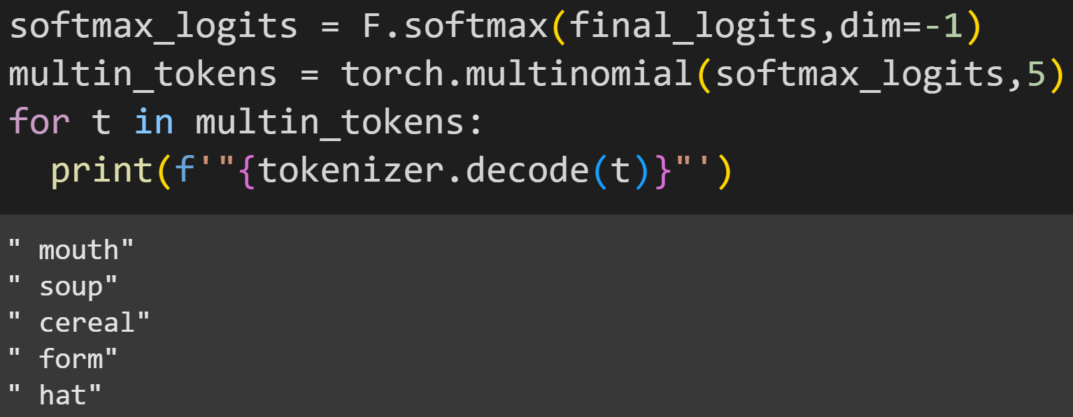
Each time you run the code, the five answers will be different (though you’ll often find the top 10 in that list). And now we know that GPT2 likes oat milk in its hat :P
These are not the only methods of injecting some stochasticity into token selection. Another method happens inside the softmax function by setting a parameter called temperature. I’ll talk about that more in a separate post on nuances of softmax.
Is random token selection good or bad? That depends on what you want from the model. If you want ChatGPT to write an imaginative children’s story about teddy bears in a space ship made from ice cream cones that introduces kids to principles of quantum computing, then the randomness increases the unexpectedness of token sequences, which makes it more creative. On the other hand, if you are asking ChatGPT for historical information about the Indo-China battle of 1962, then random token selection increases the risk that ChatGPT hallucinates. Obviously that’s not something you want. Finding that balance is an ongoing topic of investigation and refinement in LLMs.
Generating token sequences
Now you know how models generate one token. But ChatGPT doesn’t just generate one token, it generates a reply to your query that might have dozens or hundreds of tokens.
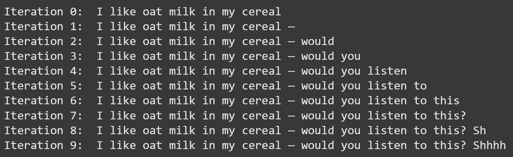
The idea of token sequence generation is simple: You input 10 tokens and the LLM generates an 11th token. Then the model inputs those 11 tokens back into itself to generate a 12th token. And so on until a specified number of tokens is generated, or until the model produces a special end-of-sequence token (that might correspond to the end of a paragraph). If you specify to generate 20 tokens, for example, then the final result will be a sequence of 30 tokens, the first 10 of which you wrote and provided as initial input, and the other 20 the model generated.
Here’s how it looks in a for-loop:
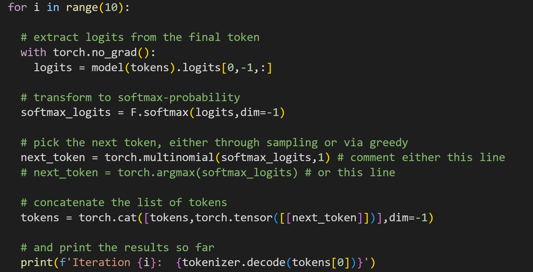
That code block has two lines to generate a next token; you can comment out one of those lines. The probabilistic selection is more interesting because it’s different each time you run the code. Here’s one gem that I got:
Seeing the implementations spelled out in code helps you understand the mechanisms, but in practice, it’s better to use the .generate method on the model object. Notice the three inputs to the generate method in the screenshot below.
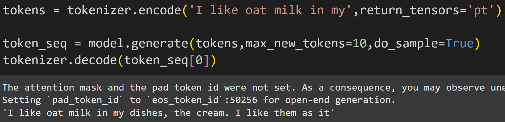
The warning message is that two additional inputs were not provided. Those are not necessary for such a simple demo with one token sequence, so the warning message can be ignored.
Please take a moment to have fun with this bit of code. Change the prompt, increase the number of new tokens, and see what happens. GPT2’s generated text is hilarious and thought-provoking.
Manipulating logits to bias token selection
So far, we have observed model outputs. The last thing I want to teach you in this post is how to manipulate model outputs. I’m going to manipulate the model’s internals to artificially inflate the logit for one token.
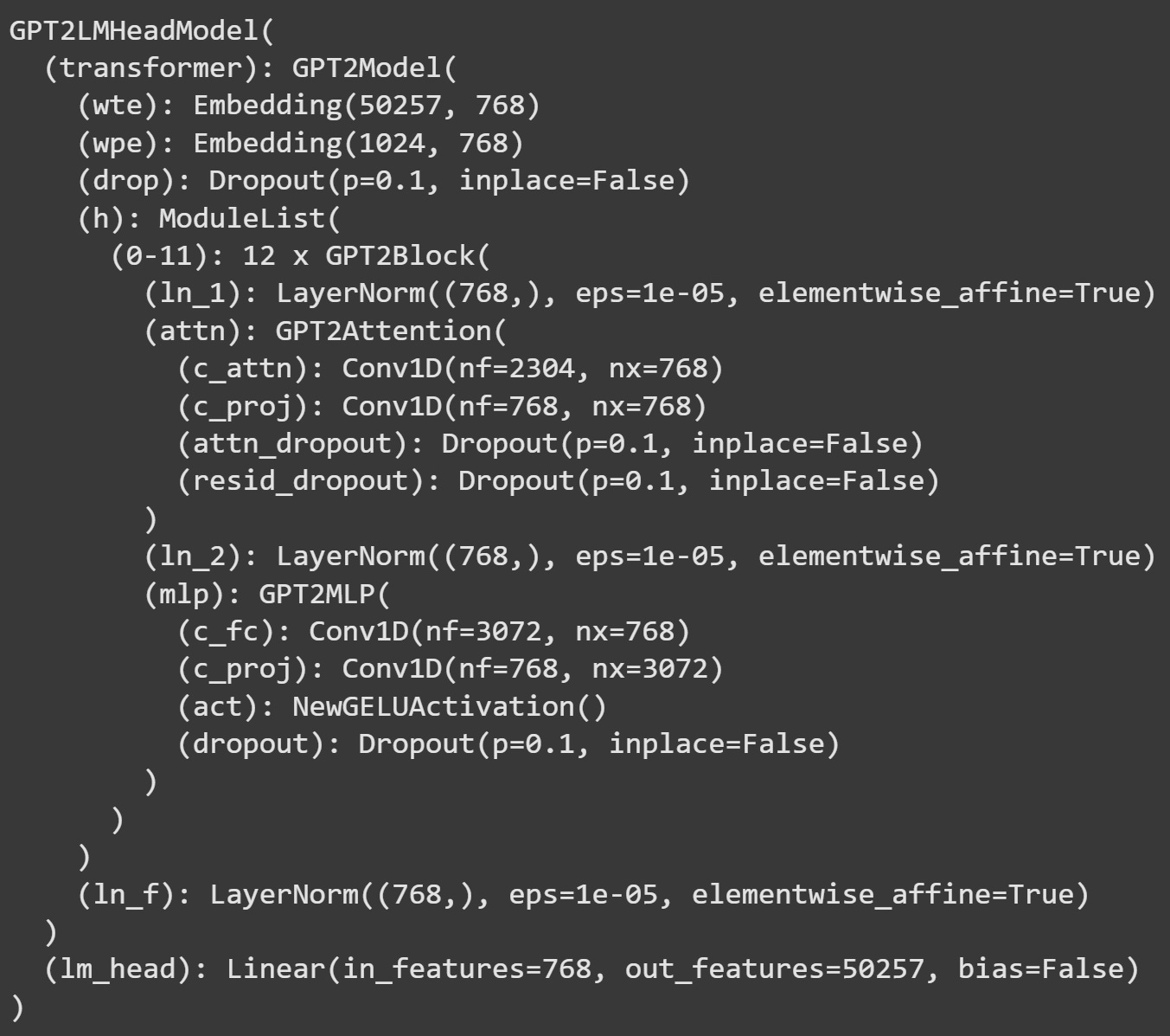
To start, here’s an overview of the model’s architecture. I will tell you about all of these layers in later posts (for example, (h) corresponds to the transformer blocks that comprise the attention and MLP subblocks); here in this post, we will only need the final layer of the model, which is called lm_model (the “head” of the language model).
The way to manipulate a PyTorch model is to implant a “hook” function into the model. That hook function allows you to interact with the model while it is processing tokens. You can use hooks to extract internal activations for later analyses (e.g., activations of individual attention head vectors) or to manipulate the activations to provide causal evidence for a specific calculation of a specific token.
Here’s what the hook function looks like. Explanations of each numbered line are below.
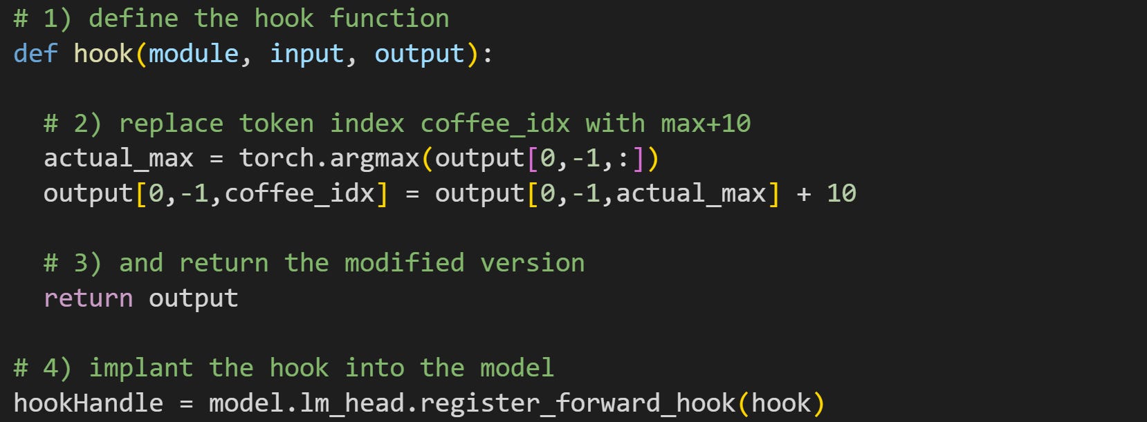
This hook function has three inputs:
moduleis a reference to the current layer of the model,inputis a tensor or tuple containing the inputs into that layer, andoutputis a tensor or tuple containing the outputs of that layer. The exact number of required inputs, and whether the variables are tuples or tensors, depend on the layer into which you implant the hook.I am overwriting one element of the output of this layer with the actual maximum token logit plus 10. This means that the token for “ coffee” will have a logit 10 units higher than the actual maximum logit calculated by the model. In other words, I am directly manipulating the output of this layer.
Just manipulating the variable inside the hook function has no impact on its own. Instead, it must be returned as an output of the function. PyTorch will replace the actual output of this layer with the modified variable
output.Here is where I “implant” the hook function into the model. I use the PyTorch method
register_forward_hookon thelm_headlayer. Getting an output from this method (variablehookHandle) allows you to remove the hook from the model if you no longer need it or want to replace it with another hook.
Now that the hook is implanted, I can run the model again on some tokens. That’s what you see in the code block below.
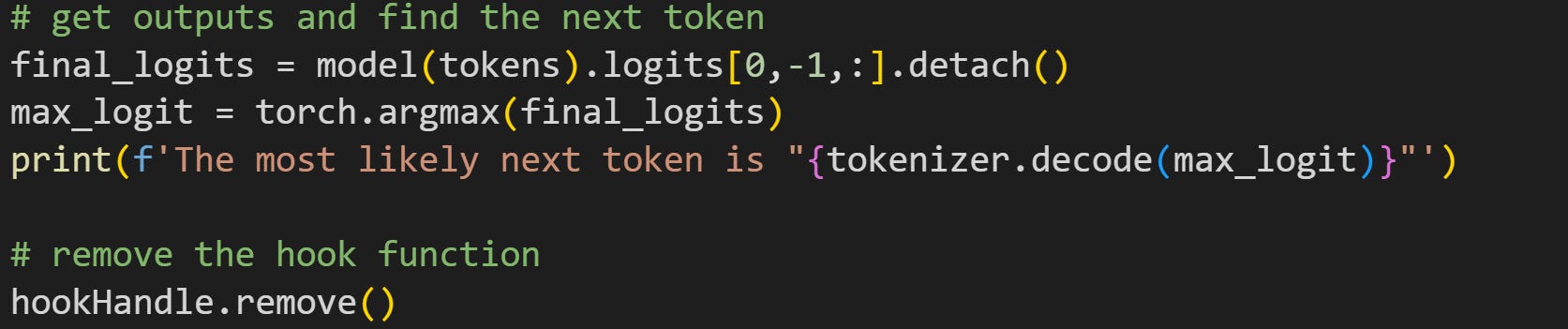
The final line shows how to remove the hook. Removing hooks is not strictly necessary; you would remove them, for example, if you’re running an experiment and want to implant a series of hooks in different parts of the model.
Figure 15 below shows the final model logits. The largest logit is now for the token “ coffee”. That is not the maximum value that the model actually calculated; that is the result of me manipulating the model’s internal dynamics.
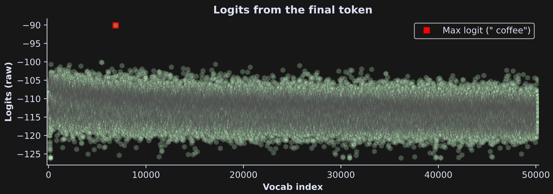
Knowing how to manipulate model internals is a fantastic tool to have in your toolkit, and we’ll continue using hook functions to measure and manipulate LLM internal activations in the rest of this series.
This Substack is human-written
I am not an AI. (I realize that an AI might write that, but I pinky-swear I’m a human.). I need to eat, pay my cell phone bill, save for retirement, and other things that responsible adults apparently do. Those things cost money.
I don’t just want your money. I want you to invest in your future by learning from educational material that I create. You can check out my video-based courses and textbooks. I hope you find that their value far exceeds the modest enrollment fee (if you use the discount coupons on my website, each course is $15-20, or comparable price in different currencies).
And if you’re specifically interested in learning about LLM structure and mechanisms, check out my 90-hour online course, which includes lectures, TONS of Python demos, and exercises and projects. Here’s a link to the course, and here’s a link to the course GitHub repo where you can download all the Python code for free, even without being in the course.