LLM breakdown 4/6: Transformer outputs (hidden states)

Transformers are the heart and soul of modern language models.

About this 6-part series

Welcome to Post #4 of this series!

The goal of this series is to demonstrate how LLMs work by analyzing their internal mechanisms (weights and activations) using machine learning.

Part 1 was about transforming text into numbers (tokenization), part 2 was about transforming the final model outputs (logits) back into text, and part 3 was about the embeddings vectors — dense representations of tokens that allow for rich contextual modulations and adjustments. Now you’re ready to start learning about the famous transformer blocks that make LLMs so impressive and capable.

Use the code! My motto is “you can learn a lot of math with a bit of code.” I encourage you to use the Python notebook that accompanies this post. The code is available on my GitHub. In addition to recreating the key analyses in this post, you can use the code to continue exploring and experimenting.

What is a transformer block?

A transformer block is a collection of calculations that analyze the input token sequence (that is, the prompt you type) and use a combination of context and world knowledge built from a ton of training data (i.e., digesting most of the Internet) to push the embeddings vectors from pointing towards the input token to pointing towards the model’s prediction of the next token.

Below is a diagram I showed in Post 2. Without the transformers, the embeddings go to the unembeddings (remember that the unembeddings are like an inverse of the embeddings), and thus, an LLM sans transformers would literally just return its input. That’s obviously not what LLMs do, so yeah, the transformers are a big deal.

Figure 1: Overview of an LLM. Without the transformer blocks, an LLM would output its input.

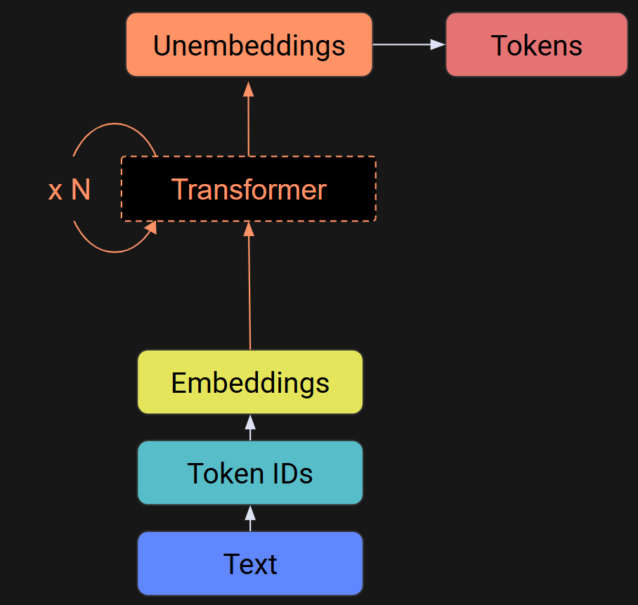
A transformer block has two sublayers (plus a few normalizations): attention and MLP (multilayer perceptron). There is a detailed diagram below, but do not freak out about it. It looks very complicated, but I’m going to explain it in detail over the next two posts. For now, I just want you to see what the internal mechanics look like.

Figure 2: Diagram of the inside of a transformer block. This post is just about the output of the block, and the next two posts are about the two sublayers.

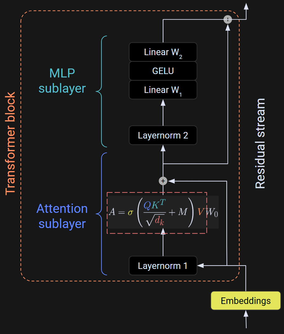
The focus of this post is the output of the transformer block — the white array at the very top of Figure 2. And what is that output? It’s the embeddings vectors that you learned about in the previous post, with the adjustments (transformations) calculated by the internals of the transformer block. So, each transformer block transforms the embeddings vectors by a little bit. After dozens of transformations, the embeddings vector from one token points to a different token that the model predicts should come next.

The outputs of the transformer blocks are also called the “hidden states” of the model.

Python demo 1: Inspecting hidden states

I am a huge fan of learning by coding. The online code notebook for this post is on my GitHub repo. You don’t need to follow along with the code, but if you’re comfortable with Python and you really want to learn the material, then the code is a fantastic supplement to this text.

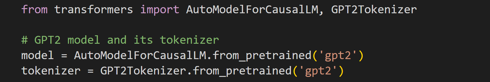
We start by importing a model and its tokenizer. I’ll continue using GPT2, partly because it’s often used when learning about LLMs, and partly to maintain consistency with the other posts in this series. You’ve seen the code below in the previous post.

There is something new I’d like to introduce to you: model.config. That is a configuration JSON that includes summary information about the model architecture, such as the number of transformer blocks (n_layer), embeddings dimensionality (n_embd), vocab size (not shown in the screenshot below), number of attention heads (n_head), and more.

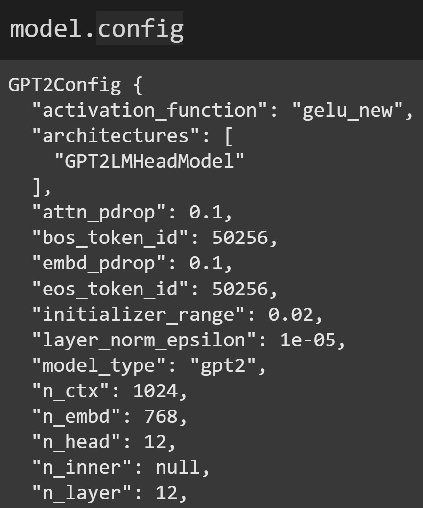
Figure 3: Some of the model properties listed under model.config.

The “hidden states” of a model are the activations that arise during a forward pass. They reflect a combination of the model’s millions-to-billions of learned parameters (which are fixed after training) and the prompt given to the model. This means that we cannot extract hidden states without the model processing text. And how do we extract the hidden states? In previous posts you learned about “hook” functions that we implant into the model. We can implant hooks to get the hidden states, although the HuggingFace models have an optional output that returns the hidden states without implanting a hook.

But first: the tokens.

Figure 4: Screenshot of tokens used in this demo, with a slightly different syntax.

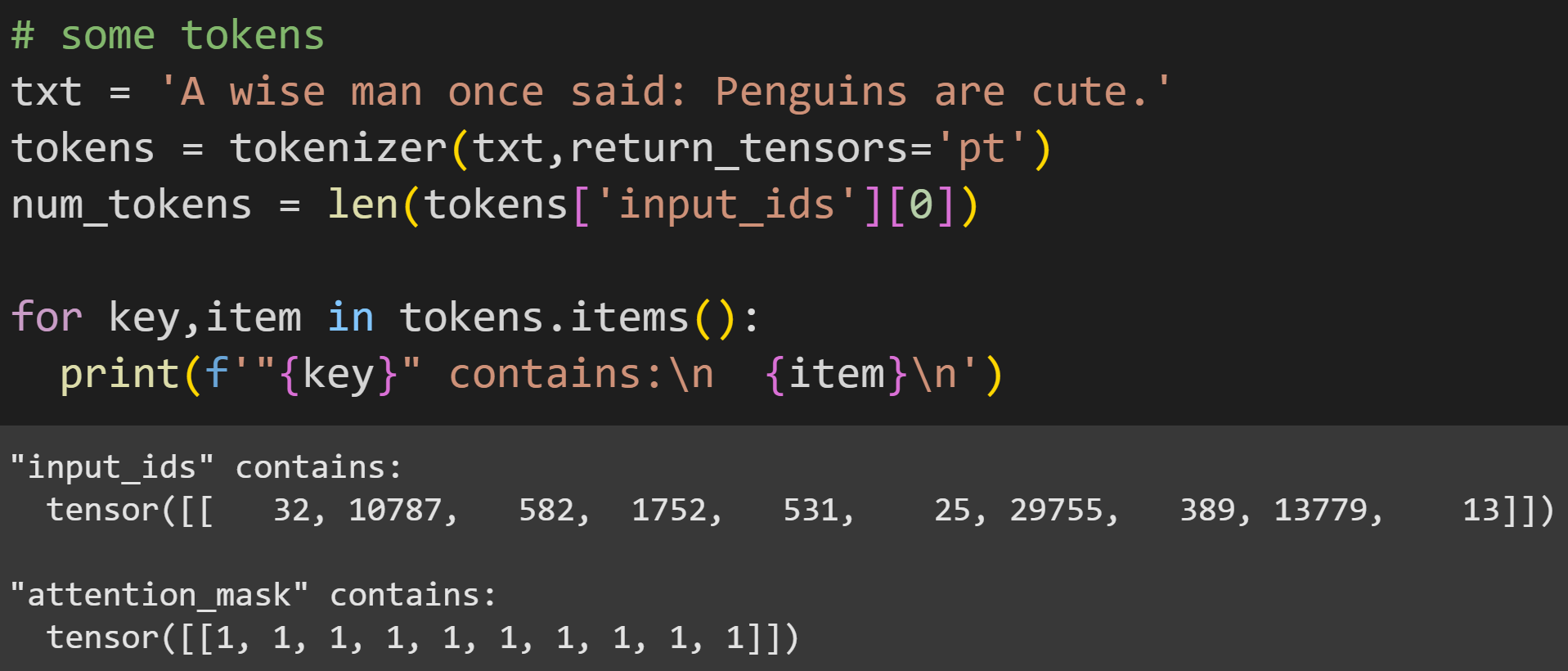
In previous posts, I used syntax like tokenizer.encode(txt) and the output was a PyTorch tensor of integers. Here, however, I don’t call a method but instead call the entire tokenizer object. That gives a different output — a dictionary with input_ids containing the token indices, and attention_mask containing all 1’s. The attention mask is used only if you input multiple text segments to process in parallel, and if those segments have different lengths. That is not relevant for this post, but I wanted to show some additional ways of using the tokenizer that would be relevant if you continue learning about LLMs mechanics.

Anyway, now we can push the tokens through the model. In previous posts, I used the syntax model(tokens). However, here there are two changes: The first is to unpack the tokens dictionary (this is necessary if you use the tokenizer as I showed above); and the second is to request that the model output the hidden states. That puts new keys into the outputs variable, as you see here:

Figure 5: Screenshot of calling the model and inspecting the hidden states sizes.

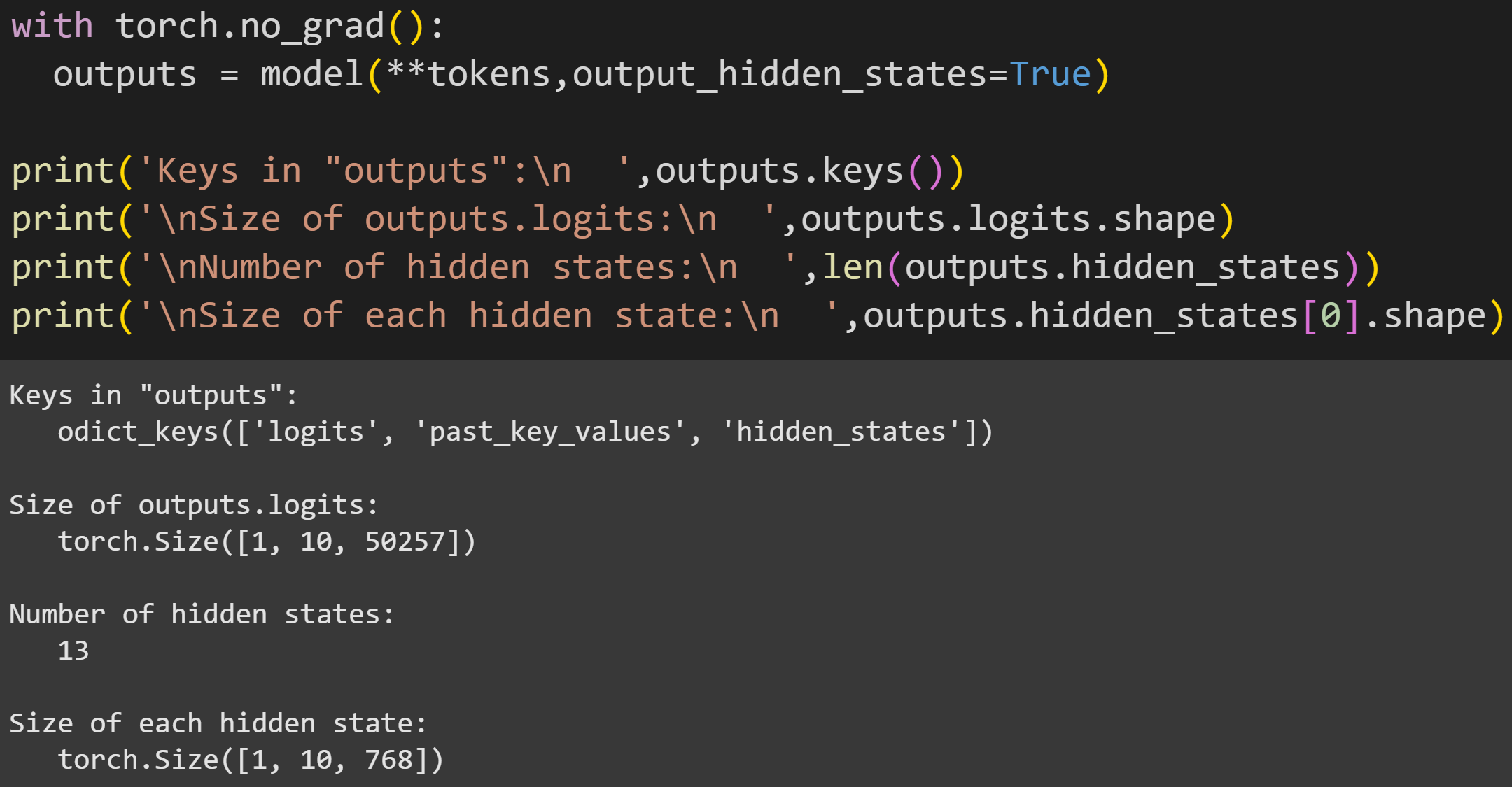
There are 13 hidden states. Does that seem… wrong? I wrote that the hidden states are the outputs of the transformer blocks, and there are 12 transformer blocks.

Well, the hidden_states variable additionally includes the token embeddings in the first element. Thus, one embeddings + 12 transformers = 13 tensors. (Some additional subtlety here: the hidden state of the embeddings matrix is the token embeddings plus the position embeddings. I haven’t discussed the position embeddings in this post series, but they allow the model to represent the positional distance between tokens in a sequence.)

Each hidden state is a tensor of size 1x10x768. The first dimension corresponds to batches (multiple text sequences processed in parallel), the second is the number of tokens in the sequence, and the third is the embeddings dimensionality.

As I wrote in the previous post and in the beginning of this post, the entire purpose of the transformer block is to calculate small adjustments to each token embeddings vector; hence, the token vectors preserve the embeddings dimensionality from the start to the end of the model.

There’s one visualization for Demo 1, but first I’ll define a few additional variables for convenience.

Now for the visualization. In the previous post, we visualized embeddings vectors, and the numerical range of the vectors was around |.2|. Figure 6 below shows that the numerical values of the hidden state activations generally increase as the embeddings vectors move deeper into the model.

Figure 6: Left panel shows the activations for each token in the hidden states (output of the transformer layer). First block is the embeddings vector.

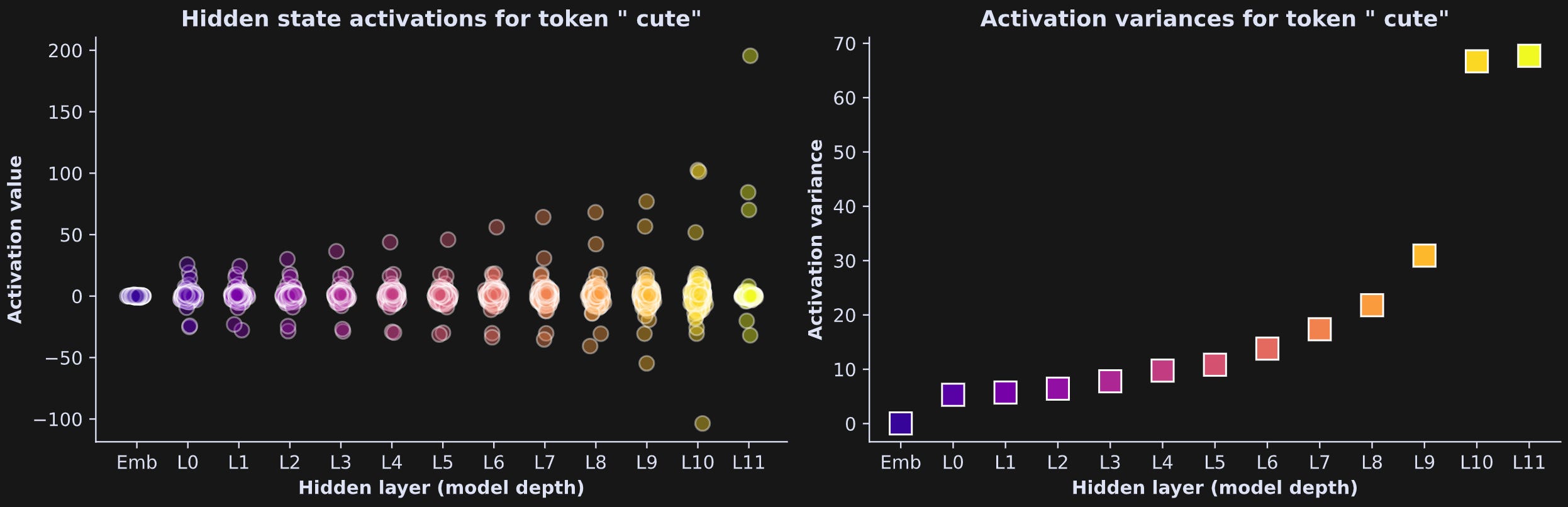
In the left panel, each dot corresponds to each of 768 embeddings dimensions, and in the right plot, each square is the variance within the layer; larger numbers indicate more differentiation across the dimensions. Geometrically, it indicates that as the embeddings go deeper into the model, they get further from the origin of the embeddings space.

Figure 6 only showed data for one token in one sentence, but it is a common observation in models like GPT2.

Python demo 2: Cosine similarities within and across layers

The goal of this demo is to explore how the token embeddings vectors relate to each other within each layer, and to the transformed versions of themselves across the layers.

There will be three visualizations in this demo.

The main statistical measure of “relatedness” is cosine similarity. I have a separate post on measuring and interpreting cosine similarity, but the short version is that it’s a number between -1 and +1 that represents the linear relationship between two variables (similar to a best-fit line between the two variables). The closer it is to 1, the more similar the two variables.

I’ll start with a single token across the layers. The idea is to pick one token, extract the hidden state for that token from all of the layers, and then calculate all pairwise cosine similarities. The result will be a matrix of cosine similarities that tells us how much the token embeddings vectors change as they pass through the model.

Pairwise cosine similarities can be calculated using PyTorch’s cosine_similarity function. The dimensions of the tensors need to line up in unintuitive ways, hence the unsqueezing in the code below (unsqueezing a tensor adds an additional singleton dimension used in broadcasting… if that sentence makes no sense, then don’t worry about it — it’s just some housekeeping that contorts the data orientation to PyTorch’s expectations).

But before we can use F.cosine_similarity, the embeddings vectors need to be isolated from each hidden state layer. Therefore, the for-loop in the code below creates a matrix of layer-by-embeddings dimension.

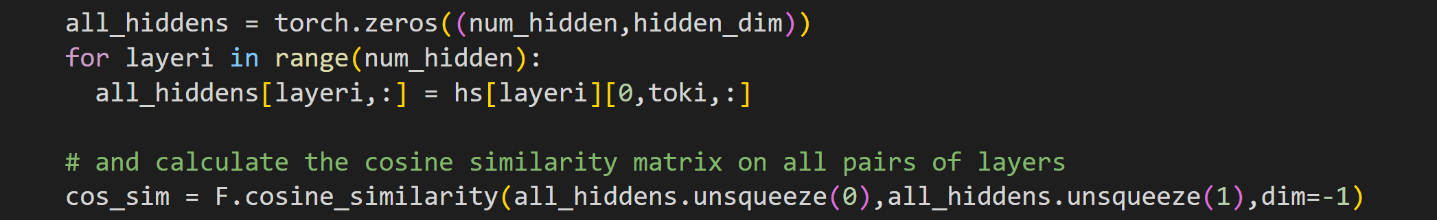
That code block calculates the cosine similarity matrix for one token (index toki). I next put that code into a for-loop over four tokens from the text. It’s really pretty to look at 🤩

Figure 7: Cosine similarity matrices for four tokens. The color of each pixel corresponds to the similarity of one token between pairs of transformer layers.

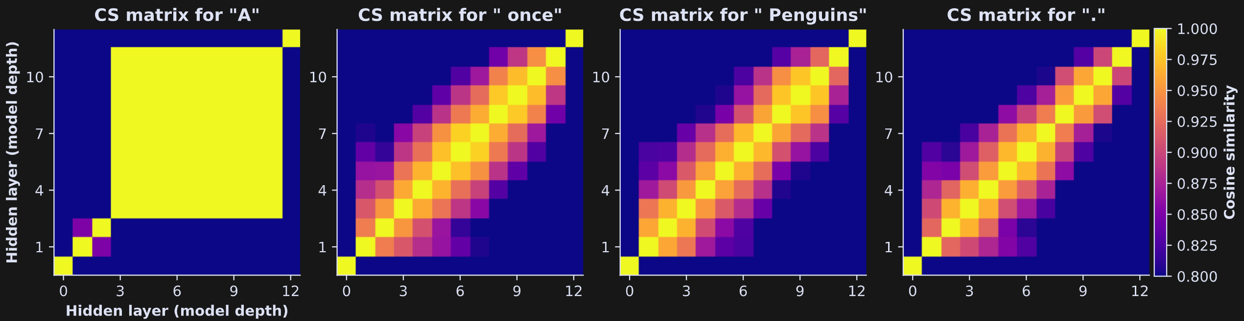
The x- and y-axes in these plots both show the hidden states layers, and the colors show the cosine similarity between each pair of layers. Values closer to 1 (yellow) indicate that the token embeddings vector is really similar between the transformer block pairs (that is, only minor adjustments to the embeddings vector).

So many interesting features of LLMs are revealed in that figure! Let’s discuss a few:

1. The first token in a sequence (left panel) is… weird. The thing about LLMs is that their entire purpose is to use the past to predict the future, but the very first token in a sequence has no past. It has no context with which to predict the next token. The activation patterns of the first token are always outliers, and should be ignored in statistical analyses. I will now focus on the other tokens.

2. The diagonal elements are all bright yellow — exactly equal to 1. Cosine similarity of a vector with itself is 1.

3. The results look overall similar, with cosine similarity decreasing further from the diagonal. That reflects that cosine similarity decreases as a function of inter-layer distance: The further away two transformer blocks, the more the embeddings change. That’s a sensible finding, but nice to see visualized.

4. The cosine similarity with the first and final layer (corresponding to the first and final row/column in the matrix) is much lower. The first layer is the token embeddings; at this point, there is no context or world knowledge that is loaded onto the vector. The first transformer block makes a big change to the vectors. The final transformer is the model’s last chance to make adjustments to the embeddings before a next-token is predicted. You’ll often see the final transformer behaving differently from the other transformer blocks. In addition, the hidden state of the last transformer includes a final normalization, which adds an additional adjustment to the vectors.

5. Although these images may look like the vectors have low cosine similarity once they get a few transformer blocks apart, check the color bar: The lowest color value is .8. That’s a really strong similarity value! Thus, the vectors don’t really change that much; I set the color scale to highlight the subtle variations. Try running the code again with the vmin parameter of imshow to 0.

Now for the second analysis.

This analysis is almost the same as the previous, but instead of tracking one token through the layers, I will calculate similarities across the tokens within a layer. Try to interpret the figure below before reading my interpretations below that.

Figure 8: Similar to the previous figure but calculating similarity across tokens within a layer.

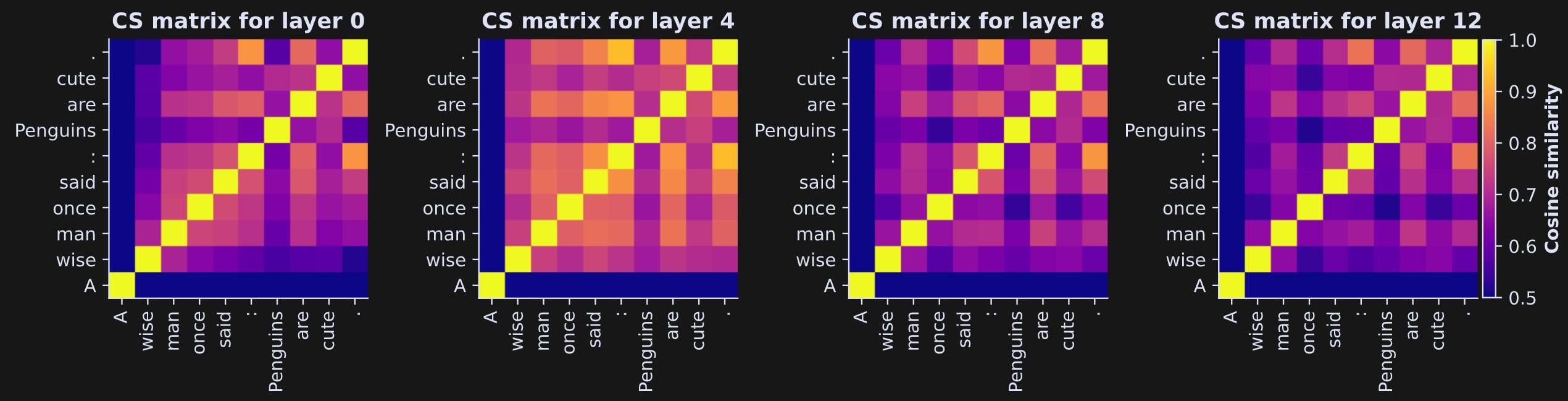
1. Again, the results for the first token (first row/column in the matrices) are very different from the rest of the tokens. LLMs just don’t have any context to work with, so analyses should exclude that first token.

2. The x- and y-axis ticks are the tokens, not the layers. So these colors correspond to the similarities of the token embeddings vectors, which is related to the clustering of token embeddings you saw in the previous post. Notice, for example, that the token pairs “:” and “.” have relatively high similarity values, whereas “Penguin” and “wise” have a low similarity (no offense to the great philosopher king penguins).

3. The cosine similarities are all positive (check the color bar). In the code, you can confirm this by setting the lower color limit to -1. In fact, nearly all embeddings vectors in GPT-style LLMs have positive cosine similarities, because the embeddings vectors are not uniformly distributed in the embeddings space, but instead cluster into a hyper-conoid. That’s a nuance of LLMs that you’d learn about in longer course on LLM mechanisms.

4. The ways that embeddings vectors relate to each other, changes across the transformer blocks. That is, the four matrices are not identical. The cosine similarity between, for example, “wise” and “cute” changes. This is what transformers do: They adjust the embeddings vectors to incorporate context and world knowledge. That’s an empirical example of something I mentioned in the previous post: The embeddings vectors are not fixed, so you shouldn’t spend too much effort trying to interpret their initial values and angles.

The final visualization I want to show here is a “laminar profile” of all pairwise token similarities across the layers. In the figure below, each little circle corresponds to the cosine similarity between a pair of embeddings vectors within each layer. It’s essentially the unique off-diagonal elements from the previous figure.

Figure 9: All the token-pair cosine similarities with each layer.

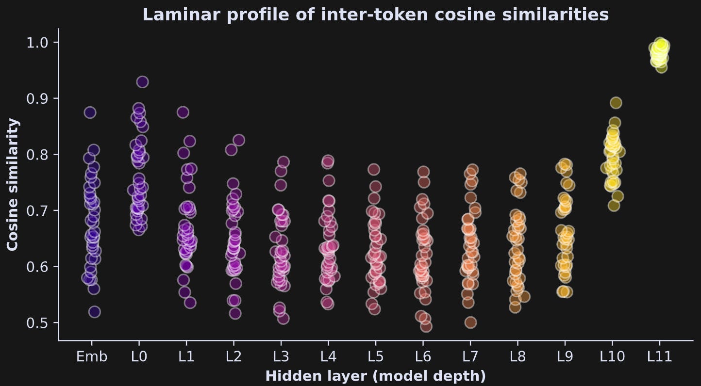
It makes a smile :)

These results show that cosine similarity across the token embeddings generally decreases around the middle layers of the model, then starts to increase again. This figure only comes from one short piece of text, but it is a common pattern of findings. The very high cosine similarities in the last transformer block are somewhat inflated by the final normalization. (btw, I have excluded the first token from this analysis; you can modify the code to see what happens when you include that pesky first token.)

Python demo 3: Manipulating hidden states

As Gregor Samsa awoke one morning from uneasy dreams, he found himself transformed in his bed into a gigantic _____

Do you know what word comes next in that quote?

Well, actually, it could be one of several words. Franz Kafka wrote The Metamorphosis in German, but it has been translated into “insect” or “bug.”¹ It’s certainly not something like “magical fairy” or “pretty unicorn that poops rainbows”.

The goal of this 3rd code demo is to manipulate the LLM’s hidden states while it processes that sentence and tries to predict the missing final token.

Let’s start by tokenizing the text.

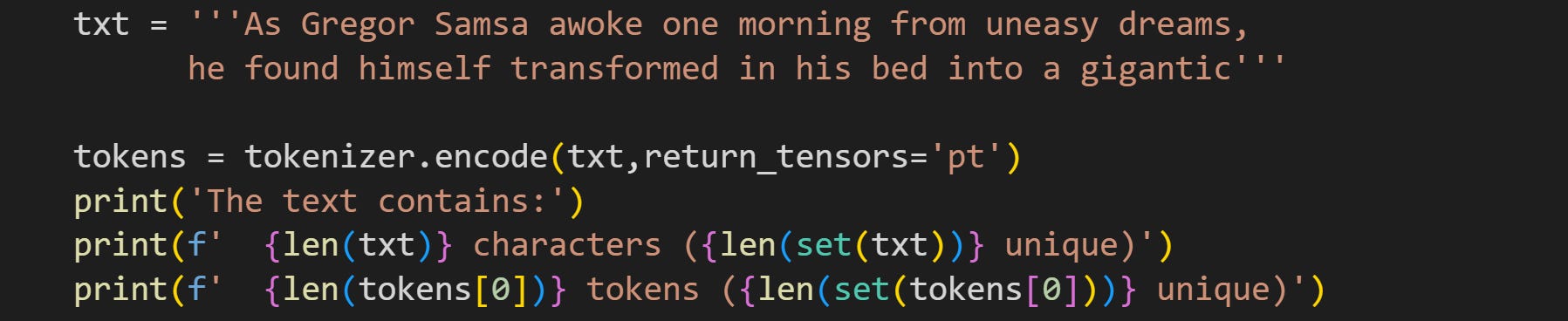
Here’s the output of that code cell:

The text contains:
  109 characters (25 unique)
  22 tokens (22 unique)

Interesting that there are so many redundant characters while no single token is repeated. Kafka really was ahead of his time ;)

Now to run a forward pass. Before doing any manipulations, I will run the tokens through a “clean” model (no implanted hooks). That provides a baseline activation that we can compare the manipulated activations against.

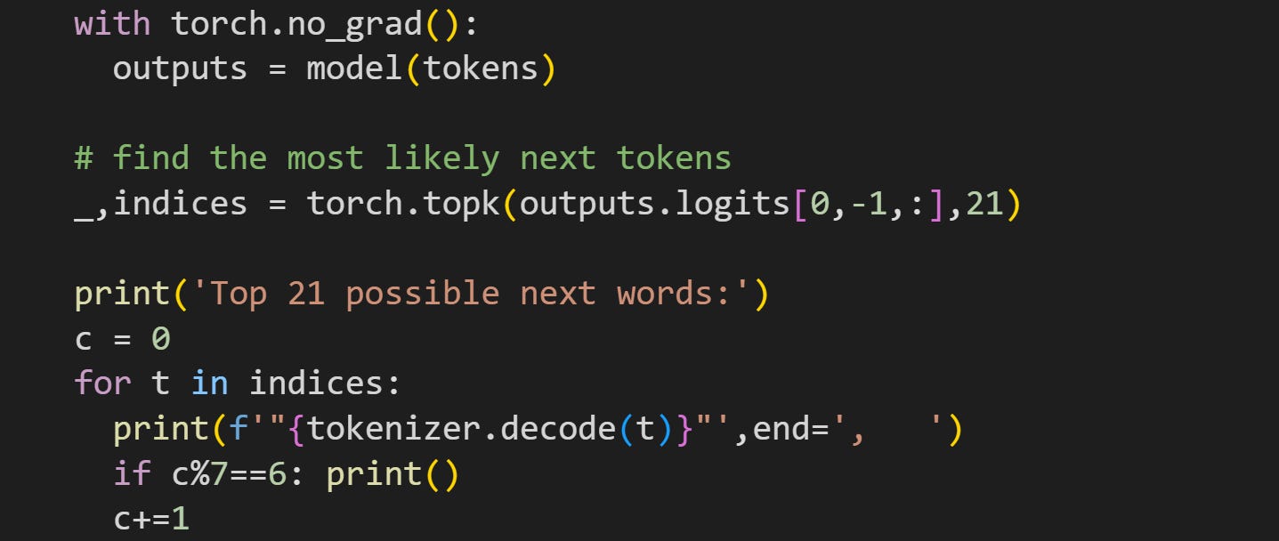
That code block pushes the tokens through the model, finds the 21 highest logits, and prints them out. Here’s what that list looks like:

Figure 10: What GPT2 thinks Gregor Samsa metamorphized into.

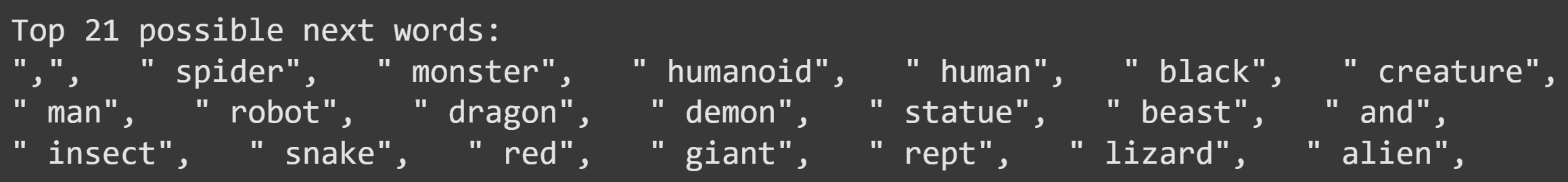
“ insect” is #15 on the list, but clearly GPT2 grasped the macabre tone of the text: all of the target words are terrifying creatures that have plagued the Earth.

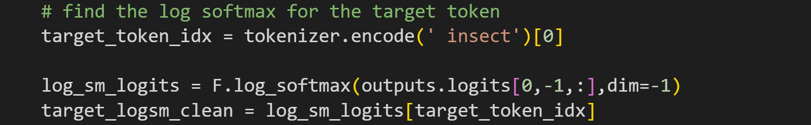
For the rest of the demo, I’m going to analyze the output logit (transformed to log-softmax) to the token “ insect”, although you can continue exploring how the experimental results look when using different target words.

The clean log-softmax value is obtained thusly:

I’ll show you the logit value in the main results figure below. First, I want to show you the code that runs the experiment. You’ve seen some elements of the code in previous posts, while other elements are new. Please try to make sense of each line of code before reading my explanation below.

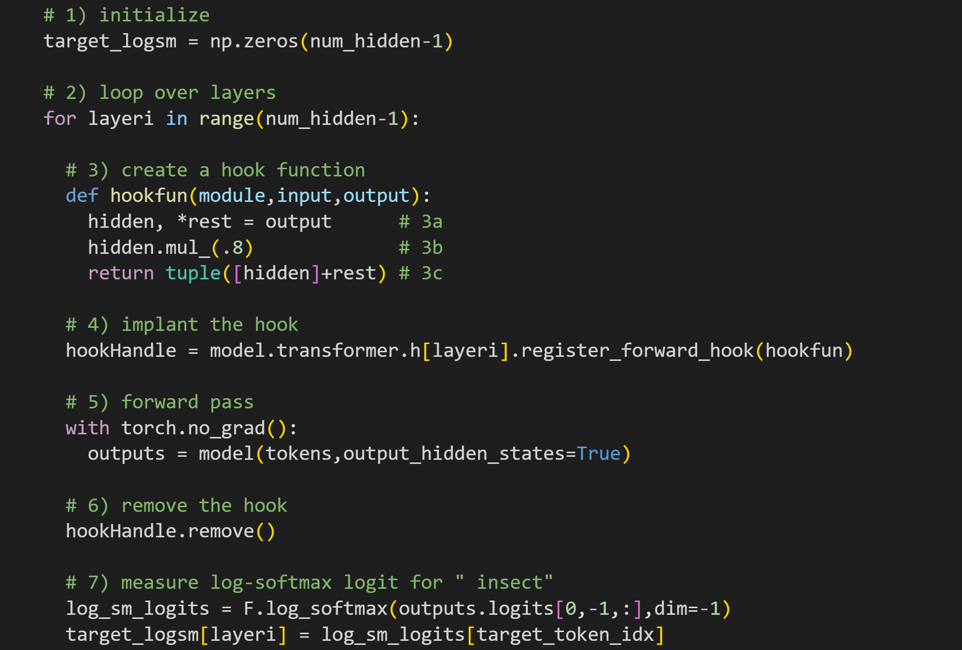
1. Initialize a vector to store the target logit values for each layer we manipulate. It is num_hidden-1 because the variable num_hidden is the number of hidden layers, which is the number of transformer blocks plus the embeddings layer. I’m only manipulating the transformer blocks in this experiment.

2. Loop over all the transformer blocks, again using num_hidden-1

3. Create a hook function. This is different from the hook functions in the previous few posts, because here we create a new hook for each layer. 3a: In the transformer blocks, the output variable is not a tensor of activation values, but a tuple in which the first element is the activations tensor (the other tuple elements are used for optional functionality that isn’t relevant here). Therefore, I unpack the first element while saving the other tuple elements for “retupling” later. 3b: Here I multiply the hidden states tensor by .8. It’s a global rescaling. This is not a targeted manipulation; literally every activation value shrinks by 20%. 3c: Here I repack the tensors into a tuple and push them out of the hook function. As you’ll remember from the previous post, that output will replace the “clean” output calculated inside the layer.

4. Implant the hook function. I’m implanting the hook into model layer h[layeri], which is the transformer block at the current iteration of the for-loop (h is for “hidden”).

5. Forward pass. I don’t actually use the hidden_states output in this experiment, but I left that output in the code in case it inspires you to explore — for example, what is the impact of scaling layer L on the hidden states of layer L+1?

6. Remove the hook. In previous posts, removing the hook was unnecessary, but now it really is important: We want to manipulate only one hidden layer at a time, so we need to remove each hook immediately after the forward pass.

7. Here is the main dependent variable. I log-softmax transform the model’s final output logits from the final token (which is its prediction for the next token), and then measure the log-softmax value of the target token (“ insect”).

And here’s what the results look like:

Figure 11: Results of the experiment. The x-axis is the manipulated transformer block, and the y-axis is the log-softmax prediction from the model output for the target word “ insect”. White dashed line is the logit from the “clean” (non-manipulated) model.

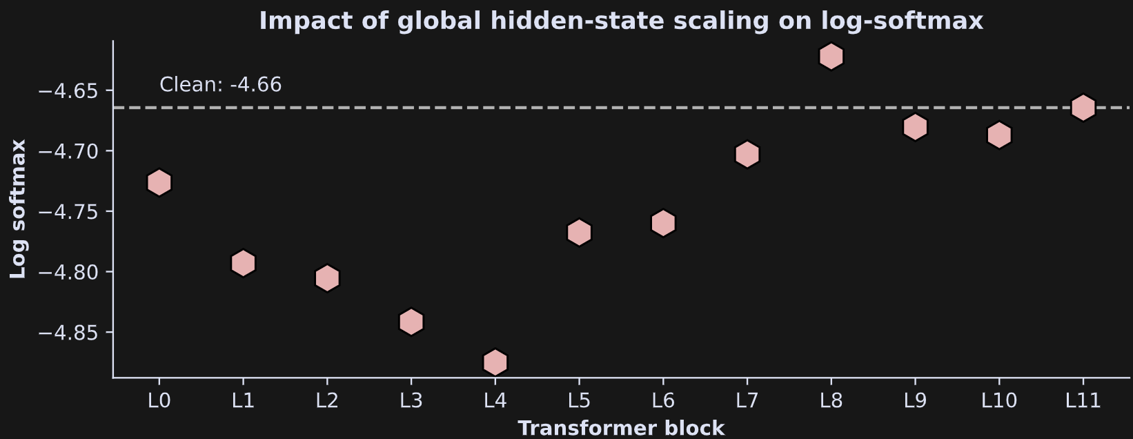
The layer-specific global scaling had an overall negative impact on the model’s ability to predict the subsequent token. A brief explanation of why this happens is that the global scaling compresses (reduces the variability of) the entire token probability distribution.

There’s so much more we could do to extend this simple experiment! But I think I’ll leave it here.

If you want to continue learning about using machine-learning and experimental manipulations to understand LLM architecture and mechanisms, consider checking out my full-length online course.

My personal transformation

I spent my entire adult life in academia until a few years ago. I was a PhD student, then a postdoc, junior faculty, and tenured professor. I ran a neuroscience research lab focusing on really technical, data-intensive, and obscure topics in systems and cognitive neuroscience.

And then I quit.

Since then, I’ve been running my company and focusing on making high-quality education widely available for low cost. If you think I should keep doing this, then please support me. But don’t just give me money — invest in your own education by enrolling in my online courses or buying my books. Those royalties will help me buy coffee that fuel posts like this. And if your finances are tight, then I’m grateful if you share my links with your BFFs from high school.

1. The opening line is: Als Gregor Samsa eines Morgens aus unruhigen Träumen erwachte, fand er sich in seinem Bett zu einem ungeheuren Ungeziefer verwandelt. The German word Ungeziefer can translate to insect, pest, bug, or vermin.