LLM breakdown 5/6: Attention

The attention algorithm that transformed AI is at your Pythonic fingertips.

About this 6-part series

Welcome to Post #5 of this series! You’re nearly at the end :)

The goal of this series is to demonstrate how LLMs work by analyzing their internal mechanisms (weights and activations) using machine learning.

Part 1 was about transforming text into numbers (tokenization), part 2 was about transforming the final model outputs (logits) back into text, part 3 was about the embeddings vectors that allow for rich context-based representations and adjustments of tokens, and part 4 was about the “hidden states,” which are the outputs of the transformer blocks. Now you’re ready to learn about the internal calculations that take place inside the transformer block, including the famous “attention” algorithm that brought language models from academic curiosities to the most powerful form of tech that humans have (so far) produced.

Use the code! My motto is “you can learn a lot of math with a bit of code.” I encourage you to use the Python notebook that accompanies this post. The code is available on my GitHub. In addition to recreating the key analyses in this post, you can use the code to continue exploring and experimenting.

“Attention is all you need”

If you study LLMs, you need to know about this paper. This was the first publication to introduce the “Transformer” architecture, which has completely transformed the field of AI. The paper is a bit technical but not overly so; if you are comfortable with reading machine-learning papers then you’ll get through it, but if not, you might find it a challenging read. But don’t worry: In this and the next posts you will understand the internal mechanisms of the transformer block.

The title of the paper is a misnomer: attention is definitely not all you need. But the attention algorithm is elegant and powerful.

The goal of this post section is to explain the concept of the attention algorithm and its importance in LLMs. I tried to find the balance between intuition and rigor, and if you really want to get into the intricate details of the math and Python implementations, consider my longer video-based course on the topic. (Side note in case you do read the Attention paper: The modern implementation of the attention algorithm is slightly different from what they proposed in 2017, though the essence is the same.)

The figure below shows an overview of the LLM (left) and a zoom-in to the transformer block (right). Each transformer block has two main sub-parts, which are variously called sublayers or subblocks. The focus of this post is the attention sublayer, and the focus of the next post is the MLP (multilayer perceptron) sublayer.

Figure 1: Overview of an LLM (left) and the transformer block (right).

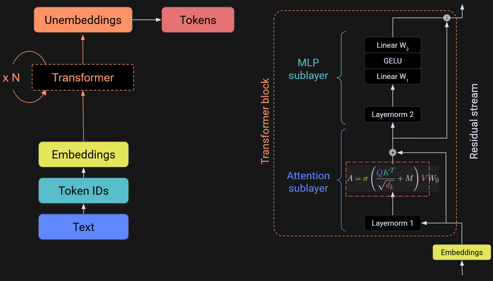
That shrunken-down equation in the attention sublayer is, like, really super-duper a lot important. It is one of the most important equations in all of modern AI. Let’s zoom in.

Figure 2: The attention algorithm (left) and how the Q, K, and V matrices are calculated as dot products between the embeddings vectors (X) and the learned weights matrices (W*).

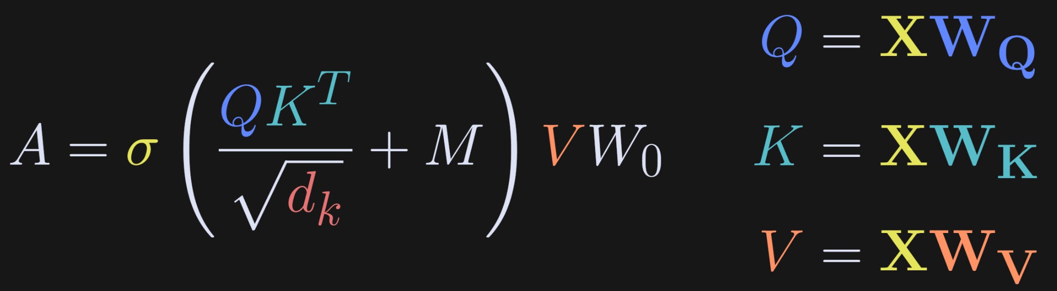
The list below explains each term in the equation, and then the rest of this post involves code demos to extract and visualize those terms.

• σ: This is the softmax function, which transforms the calculations inside into probability values.

• Q: These are called the “query” vectors. They are activations of size tokens-by-embeddings dimension, and are calculated as the multiplication of the token embeddings in matrix X, with the weights matrix W_Q. X comes from the text you put into the model, and W_Q comes from training the model, which are fixed once training is complete.

• K: These are the “keys” vectors. They have the same size as Q but come from a different weights matrix.

• sqrt(d_k): This is just a normalization factor. Matrix multiplication involves a lot of additions. That means that the range of the numbers in QK^T matrix can get so big as to cause numerical instabilities. d_k refers to the dimensionality of the attention heads, and it just scales down the dot products. I’ll say more about the attention heads later.

• That first term in the softmax function (QK^T/sqrt(d_k)) produces the “raw attention scores.” The idea is that the query vectors encode what each token is searching for, and the keys vectors encode what each token has to offer the query vectors. Imagine a dating app for embeddings vectors: Q is each token’s dating profile and K is the profile of the other tokens in the text. When there’s a good match, their dot product is high; and when there isn’t a good match (meaning the two tokens have no relevant contextual information in common), then the dot product is negative.

• M: This is a temporal-causality mask. It blanks out all future tokens, so that each token can only “match” with previous tokens (and itself), but cannot match with future tokens. That’s the mechanism that forces the LLM to use the past to predict the future. However, it is not a crucial part of LLMs. Some LLMs (like Google’s BERT model family) do not have that mask; being able to use the future to predict the present makes them better at categorizing and summarizing text, although it comes at the expense of lower performance in generating new text.

• V: These are the “values” vectors. Back to the analogy of a dating app for embeddings vectors: QK^T determines which token pairs are a good match, and then the corresponding columns in V provide the context information that adjusts the embeddings vectors. What happens to the information in Q and K? The softmax converts their dot products into probabilities. In other words, QK^T doesn’t convey information, it conveys which columns in V contain the important information.

• W0: The Q, K, and V matrices are actually concatenated “heads” that look at the same embeddings data simultaneously but attend to different features. For example, some heads extract local grammatical features (e.g., subject-verb agreement) while other heads are sensitive to longer-term context, like tagging the proper noun in the previous sentence that the pronoun “she” in the current sentence refers to. All of that disparate information from the different heads needs to be combined so that they can share what they’ve learned. The W0 matrix is called a “linear mixing matrix” because it aggregates the information from the different heads to get the final output of the attention algorithm back to the embeddings space.

Whew! There’s a lot going on in that one equation! And there are even more details and subtitles that I’ve glossed over here (although I go into much more detail about everything in my full-length course).

The TL;DR summary is this: The attention algorithm is a sequence of linear-nonlinear transformations of the text data that allow the language model to modify each embeddings vector according to contextual information from previous tokens.

Python Demo 1: Activation distributions in Q, K, and V

The main goal of this demo (using this code file) is to extract the activations from the Q, K, and V matrices from each transformer block, and visualize their distributions in histograms.

I’ll continue using GPT2, but I will switch to using GPT2-large. In the previous posts I’ve used GPT2-small. The small version has 124M parameters and the large version has 774M parameters.

Importing the large variant is nearly identical to the small variant; you just specify that you want the large version:

model = AutoModelForCausalLM.from_pretrained('gpt2-large')

The figure below shows the config file for GPT2-large. The architecture is the same as GPT2-small, but it’s both wider (more dimensions) and taller (more transformer blocks).

Figure 3: Overview of GPT2-large.

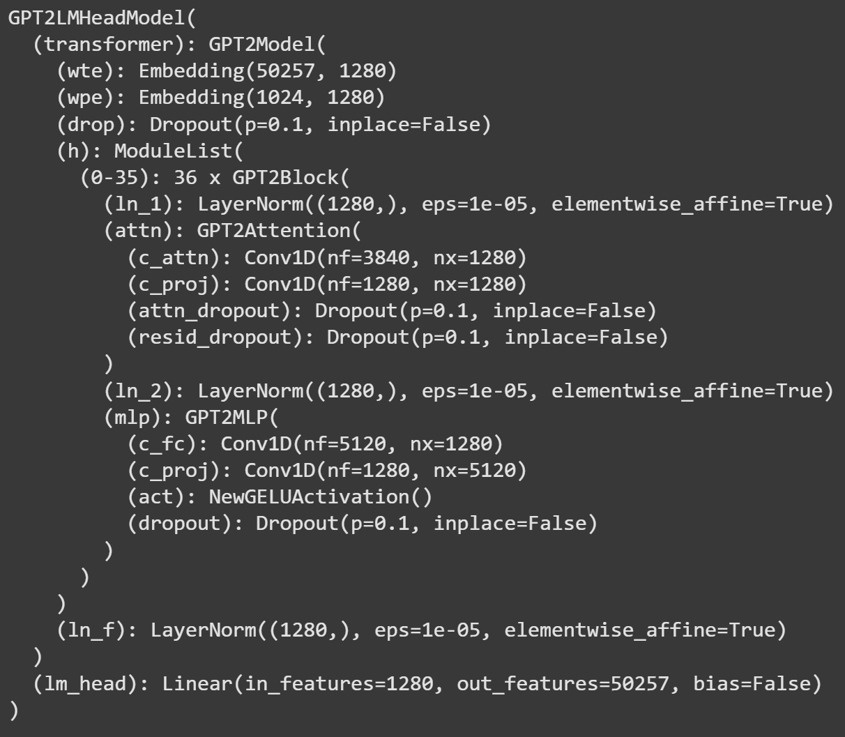
In particular, the embeddings dimensionality is 1280 (cf 768 in GPT2-small) and there are 36 transformer blocks (cf 12 in GPT2-small). Otherwise, the math and mechanics are the same for all GPT2 variants.

I want to zoom-in on the attention sublayer:

Figure 4: Feast your eyes on the attention block.

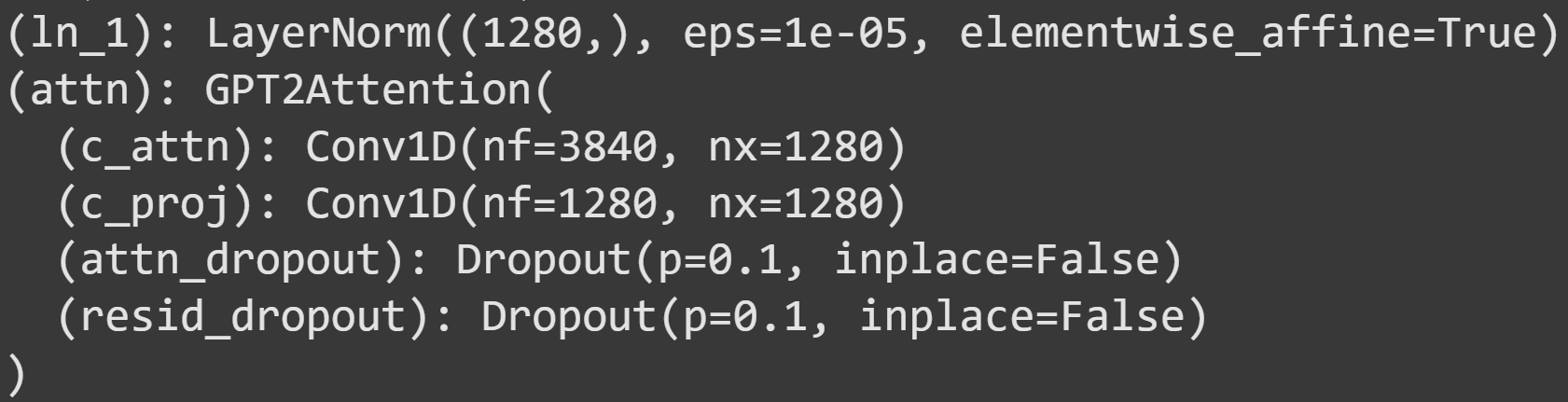
Some explanations:

• ln_1 is a pre-attention normalization. It applies a shift-and-stretch linear transformation to prevent distributional shifts. That’s more about numerical stability than any interesting calculations.

• c_attn is the main attention algorithm; it’s where the equation I showed earlier is implemented. Notice the sizes of this layer: 3840x1280. 1280 is the embeddings dimensionality, and 3840=1280x3. This is the Q, K, and V matrices concatenated into one matrix. The output of this layer is the activations that we will analyze and manipulate for the rest of this post.

• c_proj is the projection matrix, a.k.a. W0, a.k.a. the linear mixing matrix. It linearly combines all the separate things that each attention head has learned, to be sent to the MLP sublayer.

• attn_dropout and resid_dropout are regularization operations used during training. They force the model to learn more distributed representations, which makes learning more robust and numerically stable. These layers are deactivated by model.eval(), and so you don’t need to worry about them here.

Now to extract the activations by implanting hooks. There are a few differences in the code below, compared to the hook functions in previous posts.

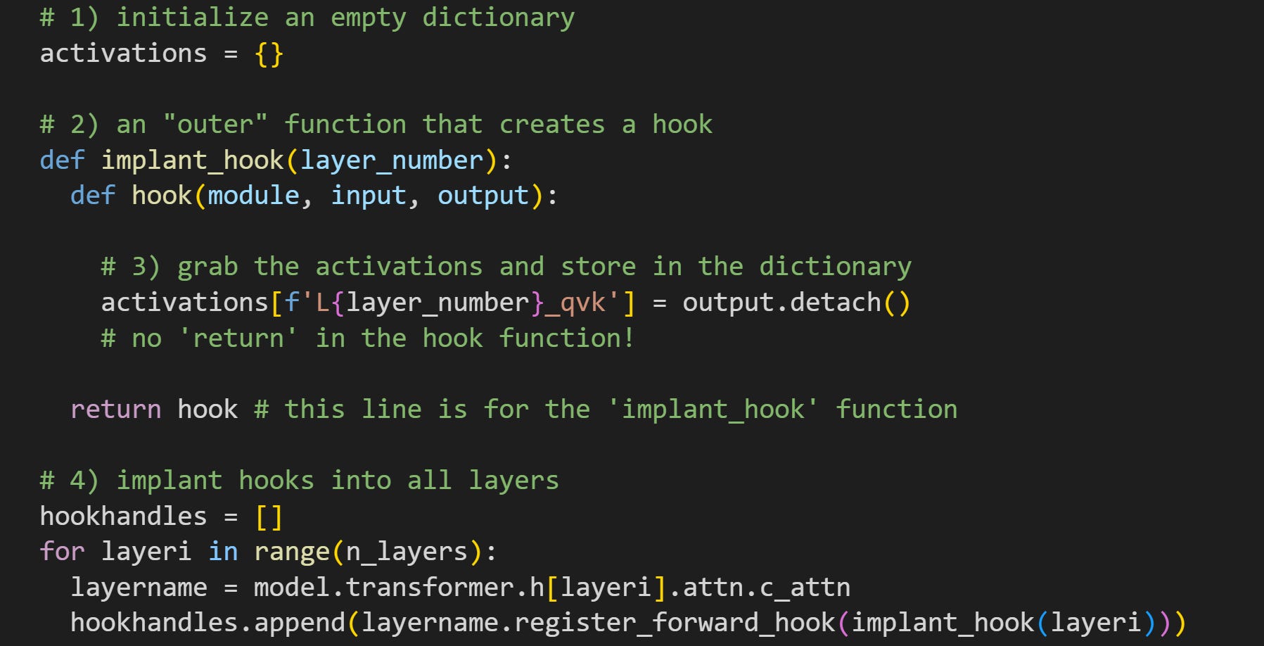
1. Each transformer block will have its own hook function, and this dictionary will store all the activations from all the layers (remember that Python dictionaries are initialized with curly brackets {} ). It’s defined outside the function, meaning it’s a global variable that will be populated inside the hook function during the forward pass.

2. There are two functions here. The “outer” function simply creates and then returns the “inner” hook function, but that “outer” function allows us to input a layer number, which in turn allows us to implant the hook into each layer and put the activations into the dictionary.

3. Here’s where I get the activations. In the previous post, I explained that the output of the transformer block is a tuple, but the output of the attention sublayer is a tensor of activations, not a tuple. I know, it’s confusing, but there are nuanced reasons for these differences, and honestly, it’s just something you get used to. The .detach() method breaks the data off the PyTorch computational graph. That prevents PyTorch from trying to track the data as we start to analyze it.

4. A for-loop over all the layers. It’s the same hook that gets implanted except for the looping index variable layeri. Notice the layer that the hooks are implanted into, with regards to the discussion around Figure 4. I’m also storing all of the hook handles in a list. In Demo 3 I will implant a new hook, and so I’ll want to eliminate these hooks. More on that later in the post!

Now that we have the hooks, we can get some data. For this demo, I’ll use one of my all-time-fav quotes from the inimitable Dr. Suess:

Sage advice indeed :)

There are 24 tokens in the text — but only 23 used in the analyses because the first token in any sequence is, as you know from the previous post, weird.

The dictionary of activations was initialized to be empty. Let’s see what happens after running a forward pass.

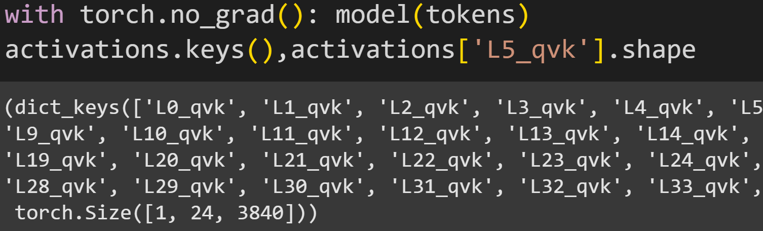
Figure 5: Screenshot of the activations dictionary after a forward pass. There are more keys to the right that are cut off.

The keys in the dictionary all have the name L*_qvk, which corresponds to the strings defined in the hook function. The bottom line shows the size of the activations from one layer: 1x24x3840. That corresponds to one text sequence, 24 tokens, and 3840, which is the Q, K, and V activations matrices concatenated into one wide matrix.

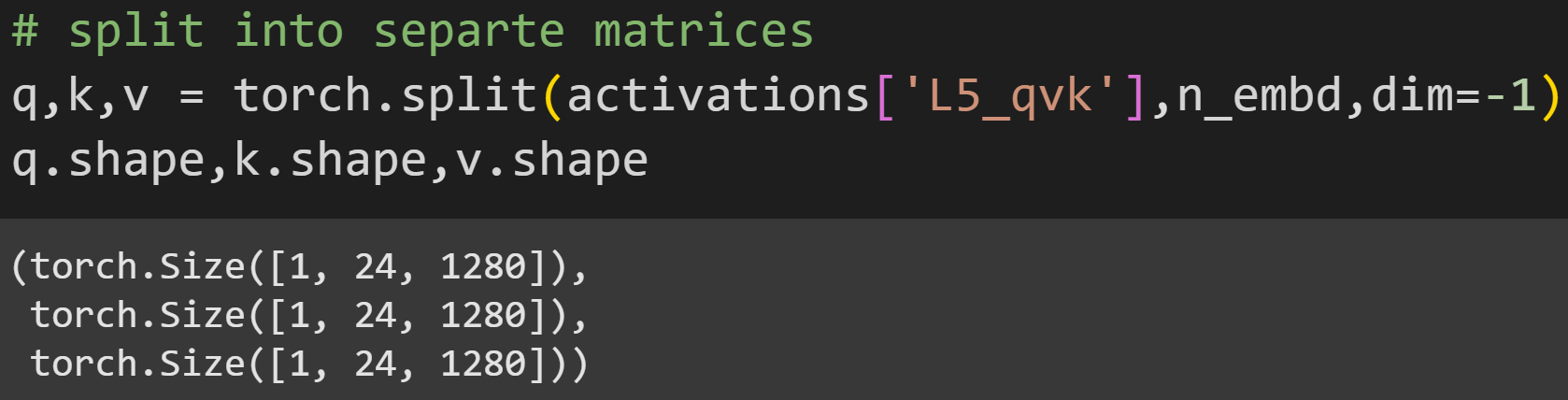
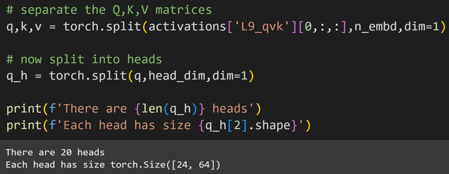
The torch.split function is a handy way to separate the matrices:

Figure 5: Separating the attention matrices.

Now to examine the data. The figure below shows histograms of all the activations from all the tokens (excluding the first) in layer 5.

Figure 6: Histograms showing the distributions of activations for the three attention matrices from one layer.

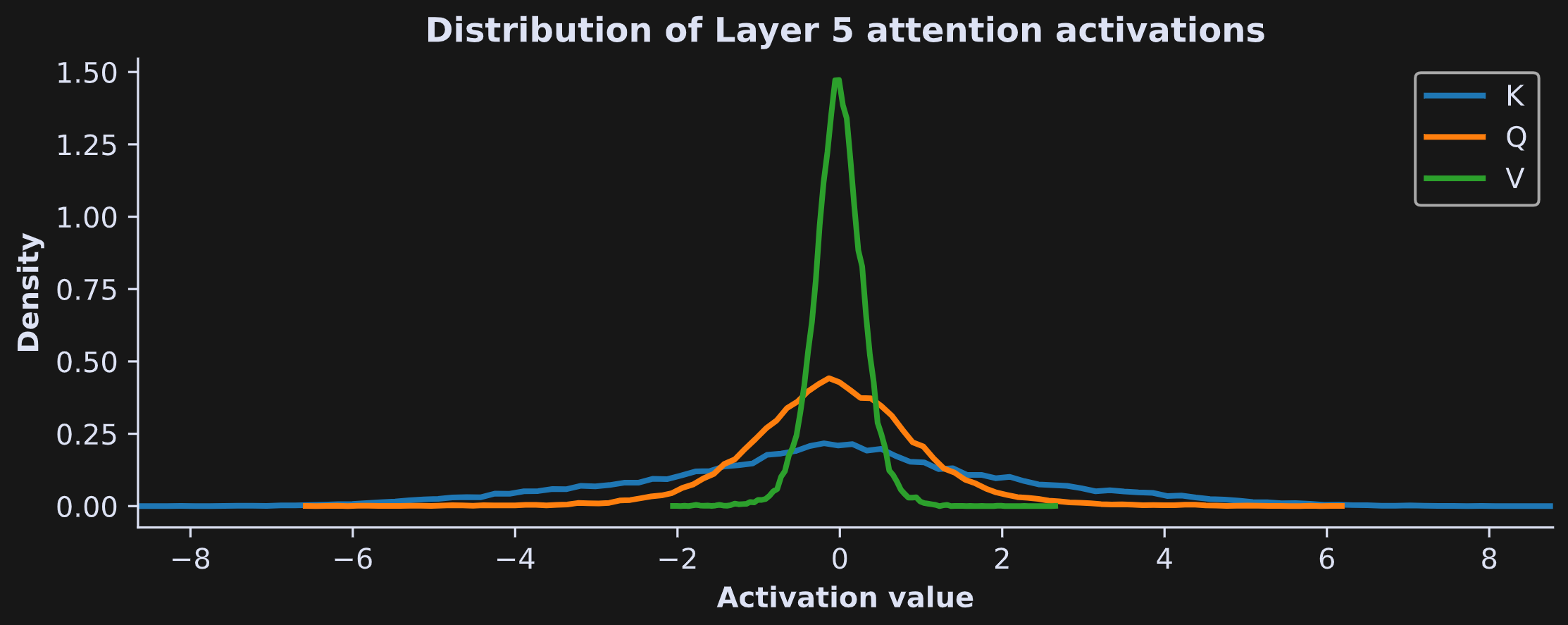
There are several interesting observations in this figure, including:

1. The activations are roughly normally distributed and centered around zero. That will be interesting to compare to the QK^T dot products in Demo 2.

2. The matrices have very different widths, with K being the widest (that is, the K activations have a lot of extreme values) and V being the narrowest (that is, most V activations are constrained to a small range close to zero).

Why did I only visualize layer 5, and do these patterns generalize to the rest of the layers? Let’s find out :D

The next analysis was to repeat those histograms in a for-loop over all 36 transformer layers. Drawing 36x3 lines is… not very easy to look at. So instead, I organized the distributions into matrices that can be visualized as images. That’s what you see in the image below: The x-axis is the activation value, the y-axis is the transformer block (higher numbers mean deeper into the model), and the color is the density — same as the y-axis in the previous figure.

Figure 7: Colormaps showing the laminar profiles of activation distributions.

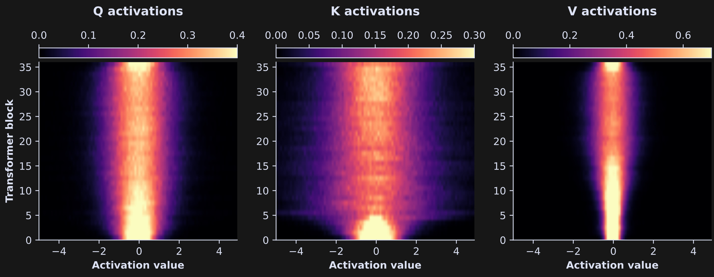
Some features are preserved, while other features weren’t visible in the previous figure. The shape of the Q activations distribution remains roughly the same throughout the model, though it thins out a bit after the first ~1/3 of the way through the model. The K activations are quite interesting: They start out very narrow, then get wider. The V activations also get a bit wider, though not as much as K. Mechanistic interpretability is a nascent field and a lot of empirical observations don’t yet have theoretical predictions or explanations, but these patterns of findings — more differentiated activations in deeper layers of the model — are consistent with the idea that the model is incorporating more varied and complex contextual information.

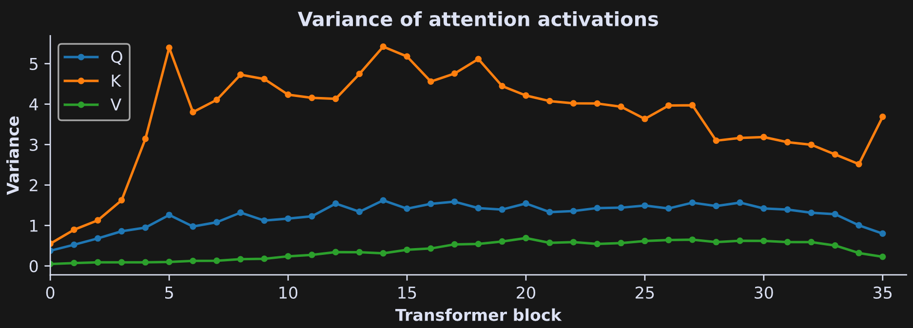
Another way to visualize the laminar profile of activations distributions is by calculating the variance of the activations within each layer:

Figure 8: Variances (how different the activations are from each other) generally increase through the LLM, indicating more differentiated and complex representations of context.

Python Demo 2: Distribution of QK^T

In the previous demo, we discovered that the Q and K activation values are normally distributed around zero. But the attention algorithm doesn’t use the individual vectors; it uses their dot products, which are compactly represented as QK^T. Are those dot products also normally distributed with a mean of zero?

Let’s find out :D

First, a reminder of the shapes of the vectors.

Figure 9: Screenshot to remind you of the sizes of the K vectors (and, by extension, the Q vectors).

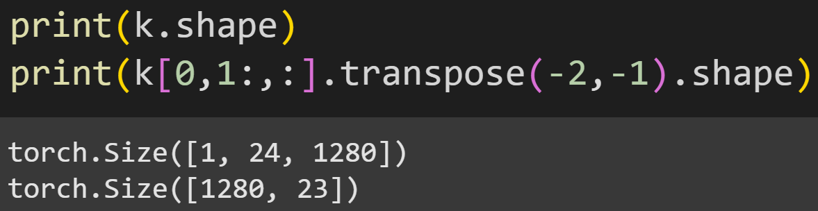
K (and also Q and V) is 1x24x1280, corresponding to one piece of text that contains 24 tokens, each of which has an embeddings dimensionality of 1280. Why do I transpose the matrix in the second line of code?

The reason is that we want to calculate the inner product between Q and K, and that matrix product is valid only if K is transposed so that the 1280 dimensionality matches. (Side note: You could avoid the transpose if you’d calculate all 24x24 dot products in a double for-loop, but that’s tedious and expensive; the matrix multiplication is more efficient.)

Now we can calculate QK^T:

Figure 10: Screenshot of the implementation and size of QK^T.

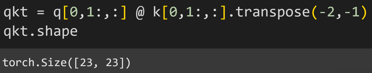
The resulting matrix is of size 23x23. What does that correspond to? It’s the dot product between each vector in Q (that is, Q’s activation to each token in the sentence) and each vector in K. The dot product is not literally the cosine similarity between Q and K, but it is the numerator of cosine similarity, and the denominator is a normalization, just like cosine similarity has a normalization in the denominator. The point is that QK^T is basically finding the similarities between Q (“I’m looking for this”) and K (“here’s what I have to offer”). Figure 11 below shows that matrix and its elements.

Figure 11: The QK^T matrix (left) and all of its elements unspooled in a scatter plot (right).

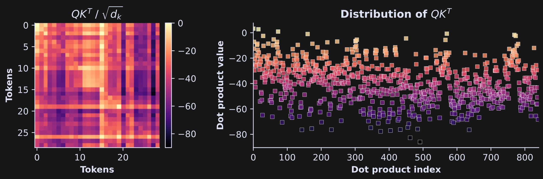
Check out that color bar — it’s all negative numbers! That’s quite surprising: Two normally distributed vectors with an average of zero have dot products that are consistently negative.

That is not some weird quirk or just chance; it is crucial to how the attention mechanism works.

Why?

I promise I’ll tell you, but I want you to think about it first. Remember that the σ() function doesn’t output the raw attention scores. Instead, it outputs the softmax-probabilities calculated on the raw attention scores. Softmax involves taking the natural exponential, which turns negative numbers into tiny positive numbers.

Below is the key figure for understanding the implications of QK^T. The left panel shows the distributions of the raw attention scores, and the right panel shows the distributions of those exact same scores but after being softmax’ed (softmaxified? softmaxerated? someone please help me with the conjugation!). Each line is from a different transformer block (see color bar on the right). Please meditate on this figure before reading my interpretations below.

Figure 12: Distributions of raw (left) and post-softmax (right) attention scores. Softmax density scores were log-transformed to highlight the small increase as p approaches 1. The distributions look “blocky” because there are so few values between the extremes.

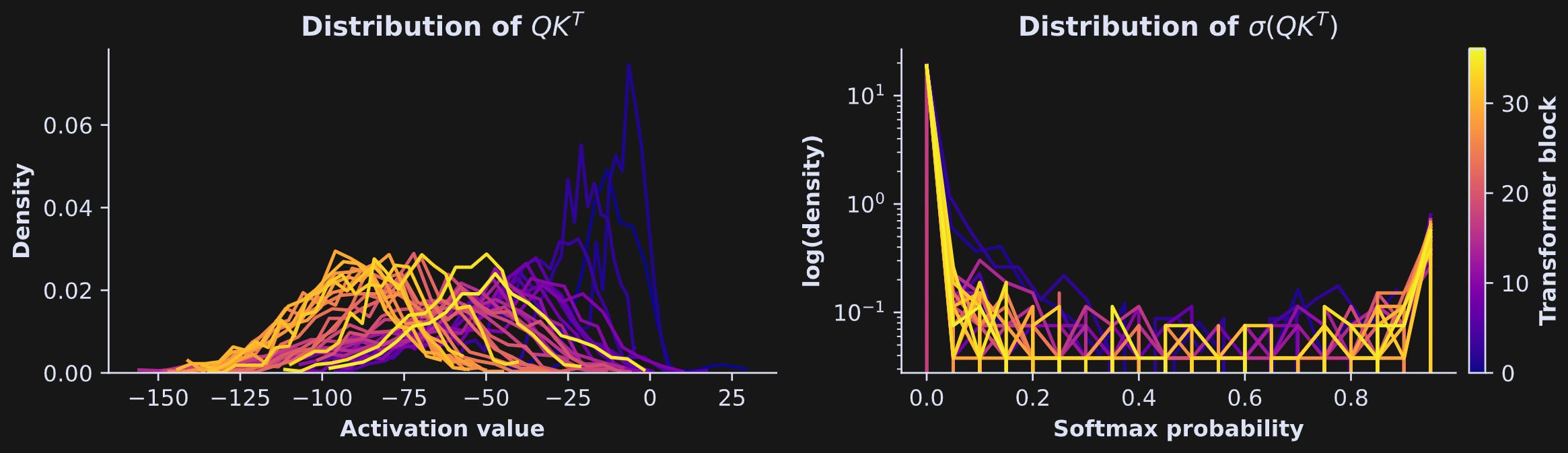
OK, here’s the deal: The goal of the attention algorithm is to pick out which tokens from the past are relevant for the future. Most tokens in the past are irrelevant for predicting the next token. Therefore, the impact of most tokens on the present token should be suppressed. That suppression is implemented by having most probabilities vanish towards zero, and allowing only a very small number of probabilities to be large. And how do you do that? By having the raw attention scores (QK^T) be mostly negative numbers! It’s really beautiful.

Another interesting feature that Figure 12 reveals is that the raw activation scores generally get more negative with increasing depth into the model. You can see that in Figure 13 below.

Figure 13. Average and standard deviation of raw attention scores across the transformer blocks. Negative distributional shifts promote sparsity after softmax.

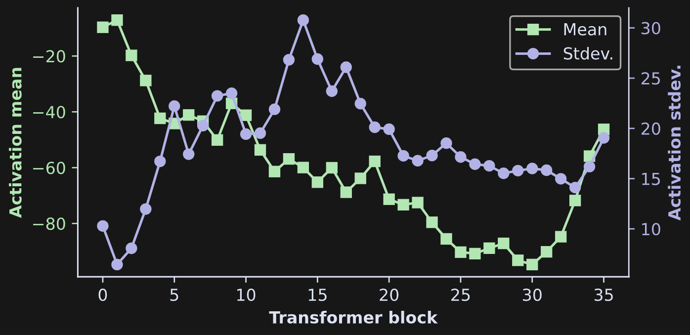
The softmax attention scores determine which columns in V get added back onto the token embeddings vectors. So, the more negative the raw attention scores, the more sparse the attention probabilities, and the more selective the attention adjustments.

Python Demo 3: Impact of attention head lesion on token prediction

I hope you’re enjoying this post so far! The last demo is to interfere with the attention mechanism, and also to introduce you to working with the attention heads.

The attention heads are computationally distinct from each other, but are concatenated into a matrix, just like how the Q, K, and V matrices are concatenated.

Figure 14: Screenshot showing how to extract individual attention heads from one layer and one attention matrix (Q in this case).

Now for the experiment.

The goal of this experiment is to zero-out (“ablate” in the parlance of LLM mechanistic interpretability) one attention head and measure the impact on the model’s final output logits. I’ll show how to ablate a head in a moment, but first we need some reference data from a clean model with no manipulations.

In some sense, we already have clean output logits from the first time I ran the model in Demo 1. However, there were hooks already implanted in the model to grab the attention activations. I want to remove those hooks. Arguably, we don’t actually need to remove those hooks, because they don’t interfere with the model calculations (except to slow things down a tiny bit, but that’s inconsequential with so few tokens). But as a minimalist with excellent dental hygiene, I like to keep myself and my LLMs clean and slim. Anyway.

for h in hookhandles:
  h.remove()

Then I ran the tokens through the clean model, log-softmax’ed the logits to the penultimate token, and examined whether the model predicted the final token. It did quite well! As a reminder, the text was:

Be who you are and say what you feel, because those who mind don't matter and those who matter don't mind

Figure 15: Log-softmax logits to the second-to-last token (“‘t”). The maximum logit, corresponding to the predicted subsequent token, is for “ mind” (red square).

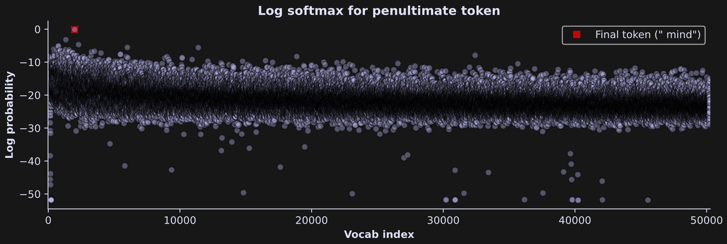
This is a fantastic result, because we can measure how that token-prediction value changes after ablating an attention head.

The experiment fits neatly into a for-loop, but it’s a relatively long loop. So I will present it over two code blocks with explanations in between.

1. The key result will be the log-softmax logit for the final token (“ mind”) measured from the penultimate token, after ablating one head in each layer.

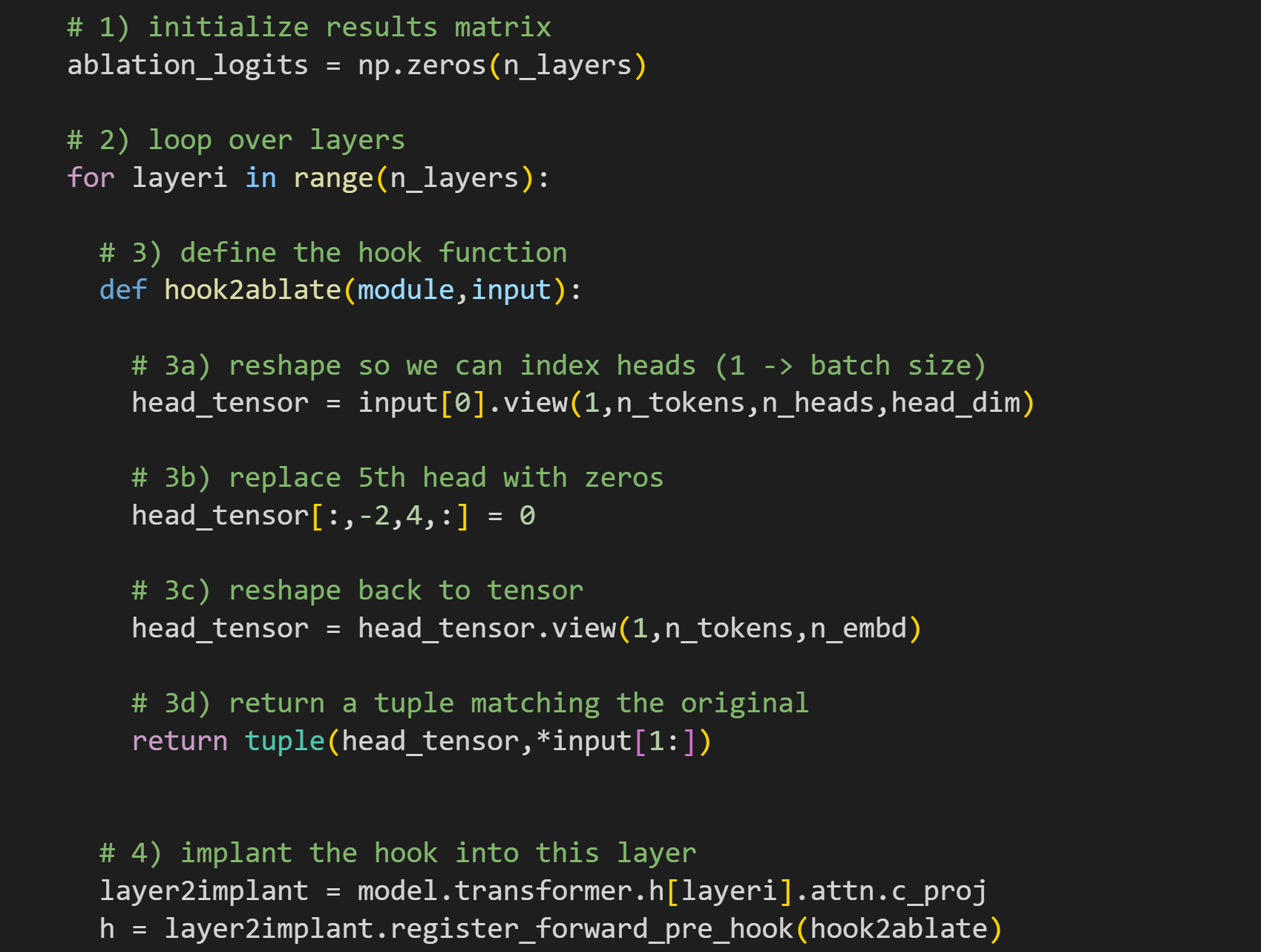
2. Loop over all 36 layers in GPT2-large.

3. Here’s the hook function. Notice that this definition has only two inputs — there’s no output variable. I’ll get back to this when I describe step 4, but you can already look ahead to see that I’m implanting a pre_hook into the c_proj layer (projection). I’m manipulating the input to the layer, not the output. This is after the attention scores are calculated (σ(QK^T)V) but before the heads get mixed by W0 and sent off to the MLP sublayer. 3a reshapes the tensor from 1x24x1280 to 1x24x20x64, corresponding to 24 tokens, 20 heads, and 64 dimensions per head. 3b replaces all the values in the 5th head with zeros (remember that zero-based indexing means that index=4 is The 5th Element), but only from the second-to-last token. We are manipulating only a very tiny piece of the model! 3c reshapes the tensor back so that the heads are all concatenated as they were before the manipulation. Finally, 3d repackages the inputs into a tuple to be returned from the function, and to replace the input that the layer actually receives. And voila! That’s how we manipulate an attention head.

4. There are two differences from the hook we used in the previous demos. First, I’m implanting into layer c_proj instead of c_attn. c_attn calculates the attention scores, and c_proj mixes them and projects them to the next sublayer. Second, the PyTorch method here is register_forward_pre_hook — note the additional pre. That means we’re implanting this hook to the input of the layer, not the output of the layer. That’s important here, because the heads are separate at the input to the c_proj layer, whereas the heads are linearly mixed by the W0 matrix at the output.

I know it’s a lot to absorb if you’re new to LLMs. Honestly, even if it doesn’t completely make sense, then I hope you have the feeling that it would make perfect sense if you spent more time on it.

Let’s continue with the rest of the experiment code. The following code block is still inside the for-loop.

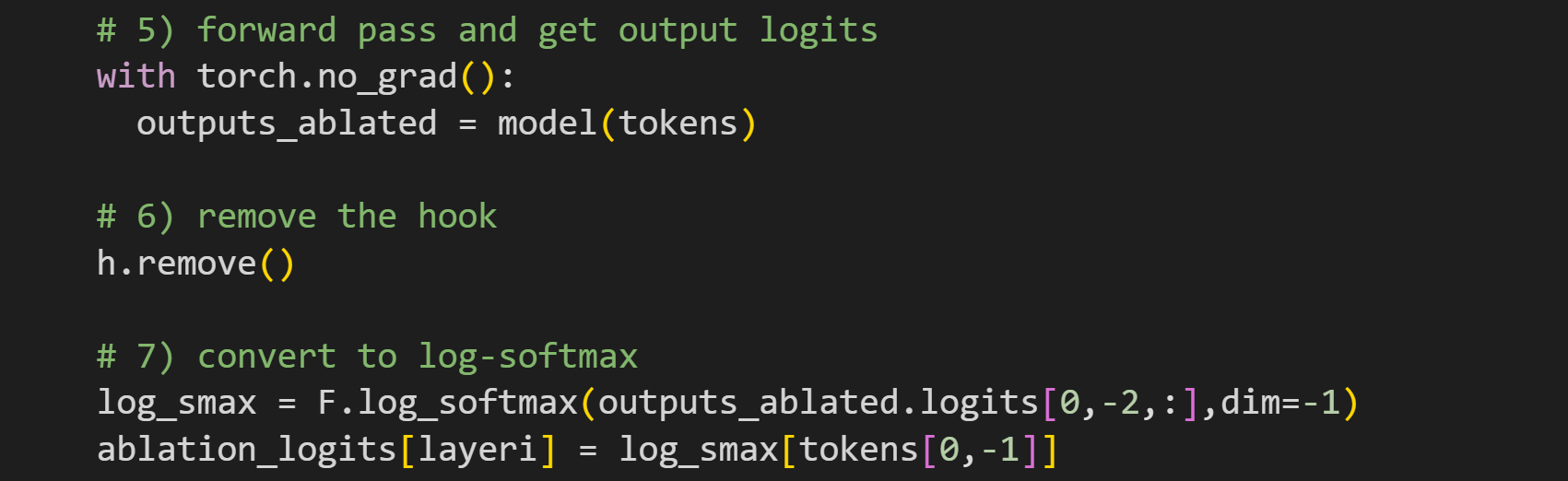
5. Forward pass. I’m pushing all the tokens through, although in the analyses I’ll only extract the logits for the second-to-last token.

6. Remove the hook. That’s important, because at each iteration of the for-loop, we only want to manipulate one layer at a time.

7. Extract the logits from the penultimate token and convert to log-softmax. These are the log-probabilities that predict the final token. The second line extracts the log-probability value of that final token.

And that’s the experiment!

Let’s see how the results look:

Figure 16: Each hexagon indicates the model output logit (log-softmax-transformed) for the token “ mind” (the actual last token in the text), after ablating the 5th attention head in each layer. White dashed line is the logit from the clean model.

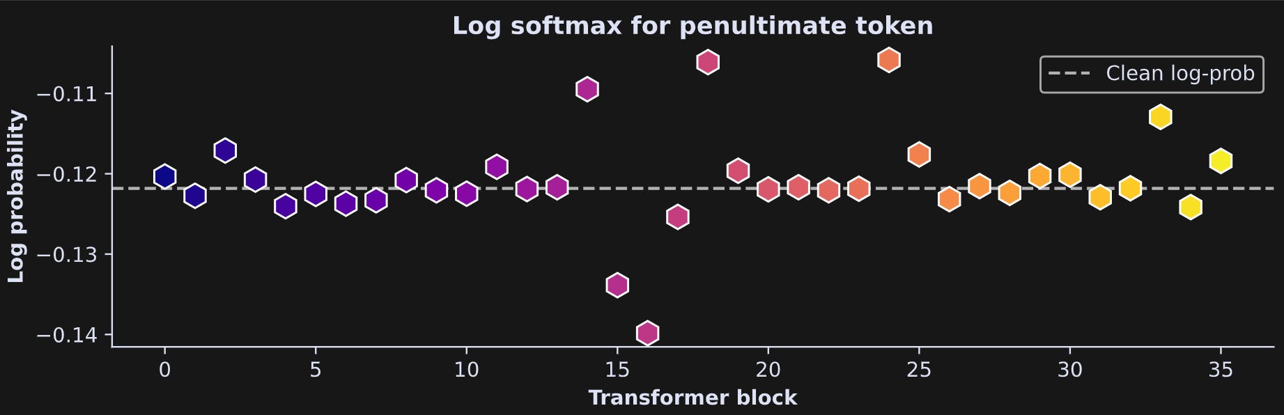
Well, it’s not a very easily interpretable result in the sense of showing a clear effect over layers. But it is obvious that this very small targeted manipulation had some impact on the final model outputs. btw, as a sanity-check that the code is correct, you can comment the line in the hook function that implements the ablation. You’ll find that all the little hexagons are exactly on the dashed line. Also btw, a log-probability of -.121 is around 89%, so the model has learned the wisdom of Dr. Suess.

LLMs aren’t difficult; they just have a lot of moving parts

Did you feel overwhelmed from this post? That feeling that you sort of, kind of, maybe are at the cusp of understanding the attention algorithm, but it’s slipping away from you even as you read this question?

Don’t be alarmed! That’s a completely normal feeling. I promise (pinky-swear) that LLM mechanisms aren’t so difficult to understand, but it takes more time and practice than just reading a few posts. If you really want to learn this stuff, then check out my semester-length online course, where you’ll get video lectures that go into more detail, with lots and lots of code demos, exercises, and projects.

One last moment of your attention

You know the routine by now: This is the part of the post where I pretend that I’m not trying to beg for money.

But I’m really not! I want you to invest in your brain (your most precious resource, even more precious than that shiny ring you found in the river), and I want you to feel that my online courses and textbooks are one of the many great ways to invest in your brain and your future.

Thank you for your attention :P