LLM breakdown 6/6: MLP

The expansion-contraction layer that opens new possibilities.

About this 6-part series

Welcome to the final post of this series! Fear not! ‘tis not the final post on LLM mechanisms, just the final post in this series.

The goal of this series is to introduce LLMs by analyzing their internal mechanisms (weights and activations) using machine learning.

Part 1 was about transforming text into numbers (tokenization), part 2 was about transforming the final model outputs (logits) back into text, part 3 was about the embeddings vectors that allow for rich context-based representations and adjustments of tokens, part 4 was about the “hidden states,” which are the outputs of the transformer blocks, and Part 5 introduced the famous “attention” algorithm. And now in this post we’ll wrap things up with the MLP sublayer.

Use the code! My motto is “you can learn a lot of math with a bit of code.” I encourage you to use the Python notebook that accompanies this post. The code is available on my GitHub. In addition to recreating the key analyses, you can use the code to continue exploring and experimenting.

A detailed video walk-through of the code is at the bottom of this post.

The MLP (or any other name)

The first sublayer of the transformer block is always called “attention,” while the second sublayer of the transformer is variously called MLP (multilayer perceptron), FFN (feedforward network), intermediate, dense, and perhaps a few other terms. I will use the term MLP to be consistent with OpenAI’s terminology and their GPT2 models. Just be aware that you might come across different labels in different models or texts.

Figure 1: Overview of an LLM (left) and the transformer block (right).

Figure 1 should look familiar from the previous post. The idea of the MLP sublayer is to take a copy of the embeddings vectors, expand their dimensionality by a factor of 4, apply a nonlinearity, and then contract the dimensionality back to the embeddings dimension.

Figure 2 below shows this in more detail.

Figure 2: Graphical overview of the MLP layer.

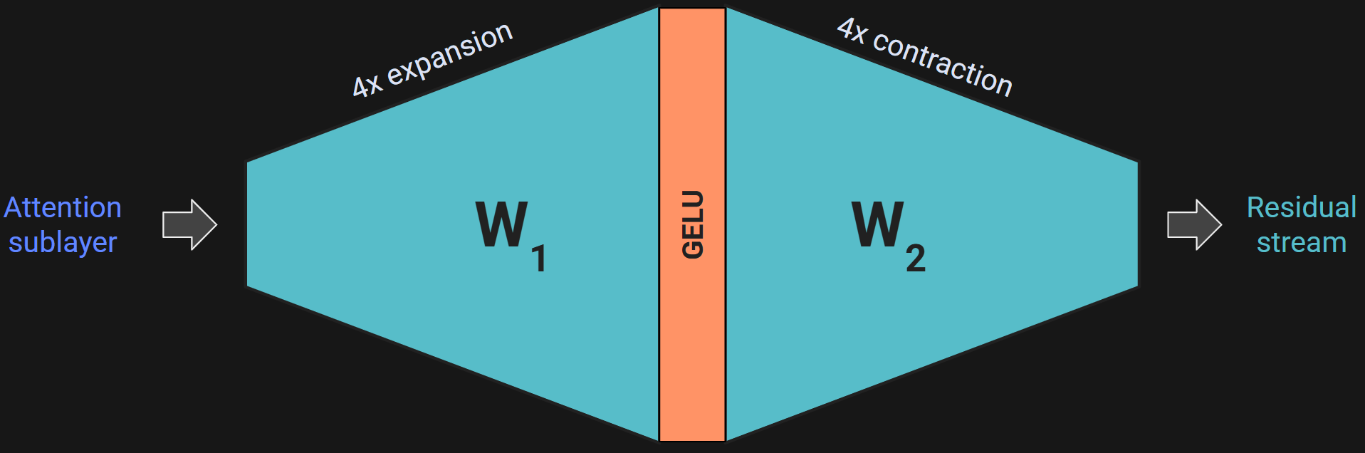
Why expand the dimensionality only to contract it one step later? The larger intermediate dimensionality creates a richer space for complex feature transformation and linear decision boundaries. I’ll unpack that in Demo 0, but the main idea is that pushing the data into a larger-dimensional space gives the model more opportunities to bind associations between different tokens, and also to incorporate world-knowledge that the model has learned but that isn’t in the currently-processed text (e.g., the model “knows” that people keep cats as pets, even if that’s not written in the prompt).

Another thing to know about the MLP layer is that all tokens are processed simultaneously; there is no cross-talk or temporal causality. Temporal causality only happens in the attention sublayer.

Demo 0: Why dimensionality expansion helps separation

Very Pythonic of me to start numbering the demos at 0 :P

But this zeroth demo is not about LLMs; instead, I want to demonstrate the idea that expanding the data dimensionality (with a nonlinear transform) allows models to identify complex features using linear decision boundaries.

Here’s the setup (and here’s the code): The goal is to separate the green circles from the red squares in Figure 3 (left) below. In 2D, that separation is impossible — if we can only use linear separators. That is, there is no straight line that separates the greens from the reds.

Figure 3: The green circles and red squares are nonlinearly separable in 2D (left), but a dimensionality expansion with a nonlinearity allows for linear separation (right).

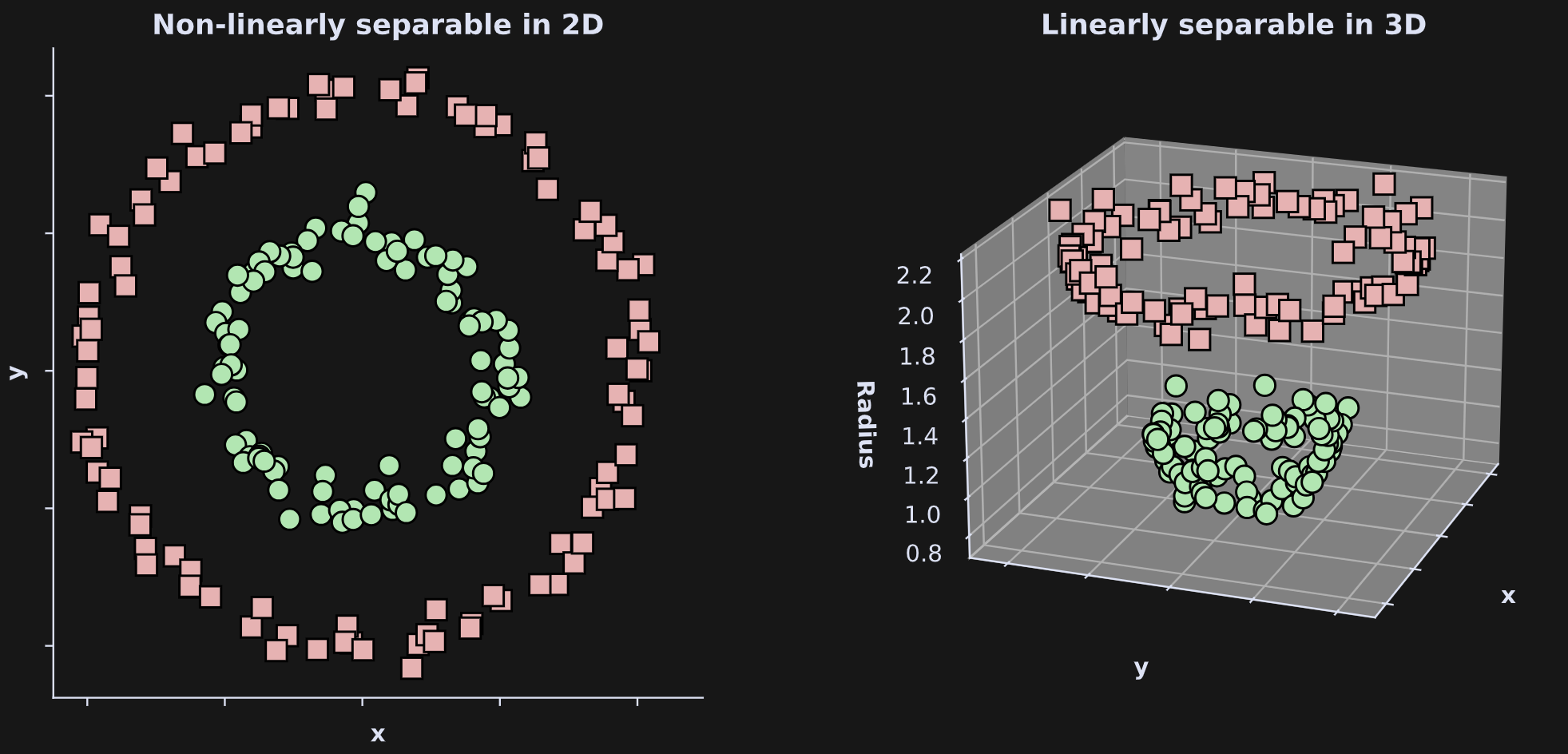
However, if we expand the dimensionality to 3D (right panel), then we can successfully linearly separate the greens and the reds (e.g., a plane in between them). How did I create that third dimension? I defined the height in the 3D axis to be the distance of each dot to the center of the graph from the 2D axis. That’s a nonlinear transform of the (x,y) coordinates.

Why is linear separation important? Linear operations (addition and multiplication) are advantageous because they are fast, numerically stable, and easily implemented on digital computers, especially on GPUs. Indeed, GPUs are literally built to make linear calculations like matrix multiplication as fast and low-energy as possible. The capability of warping a dataset into a space that facilitates linear classification makes an AI better and more efficient.

Demo 0.5: The GELU nonlinear activation function

The nonlinearity used in the MLP layer is called GELU, which stands for Gaussian Error Linear Unit. It’s similar to the ReLU nonlinear activation function used in most deep learning models, in that the positive activations pass through while the negative activations get suppressed. To illustrate the impact of this nonlinearity, I’ve created some normally distributed noise and passed it through a GELU:

x = torch.randn(4000)
x_gelu = F.gelu(x)

Figure 4 below shows the data before and after the GELU nonlinearity.

Figure 4: Impact of GELU nonlinearity on random noise data.

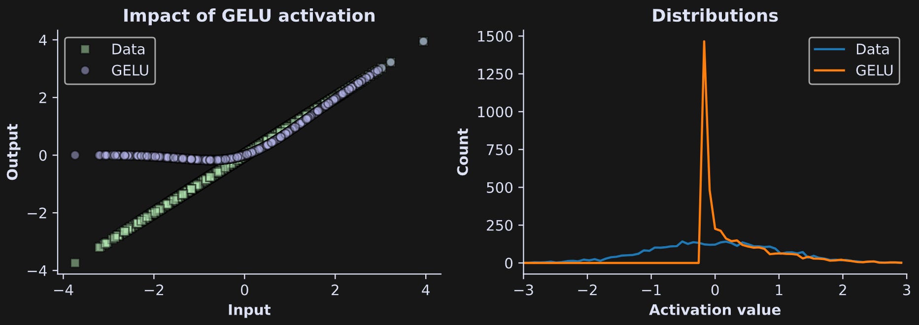
The left panel shows that the positive values of the pre-GELU activations (green squares) are preserved, while the negative values are pulled up towards zero. (Why do LLMs use GELU instead of ReLU? People have found that GELU is slightly better on really large models, and LLMs are the biggest deep learning models that currently exist.)

The histograms in the right panel show that the post-GELU activations have most of their values just below zero. That’s useful for next-token prediction, because it means that most activations are suppressed, and only a small number of activations can have a meaningful impact on the embeddings vector adjustments. As with the attention mechanism you learned about in the previous post, this means that most previous tokens have a minimal impact on predicting the next token, whereas a small number of highly relevant tokens can have an outsized impact.

Demo 1: MLP distributions before, during, and after the expansion

Let’s get back to LLMs. The goal of this first demo is to extract the MLP activations at four stages: (1) input to the MLP, (2) expanded pre-GELU, (3) expanded post-GELU, (4) contraction (the output of the MLP). That corresponds to the four vertical lines in Figure 2.

We will continue working with GPT2 models, but here I’ll switch to GPT2-medium. Just for some variety. For reference, Figure 5 below shows the transformer block architecture.

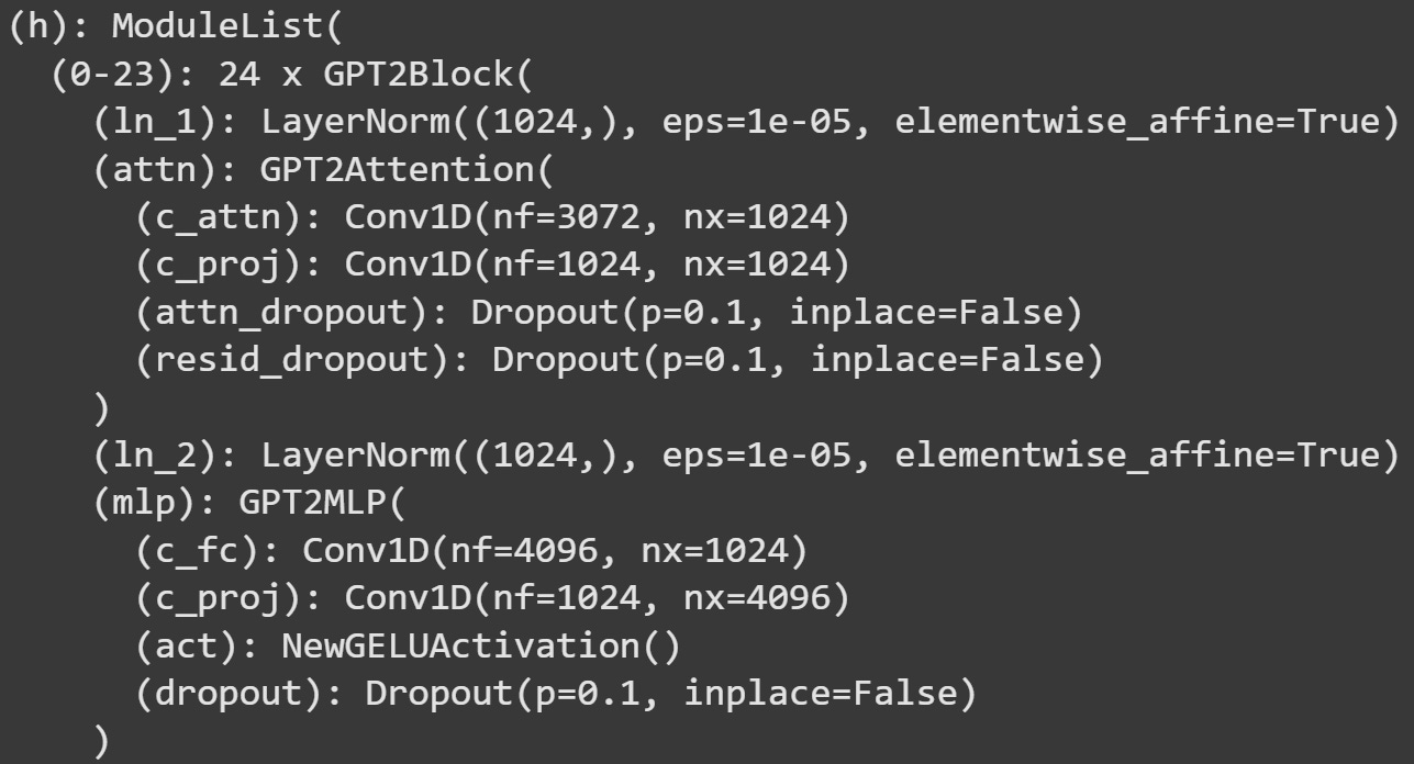
Figure 5: Overview of the model architecture. Direct your attention to the (mlp) block.

We need a hook function to extract the MLP activations. The hook function in the code block below is a little more involved than those in previous posts; please try to understand what it does and why it works, before reading my numbered comments below.

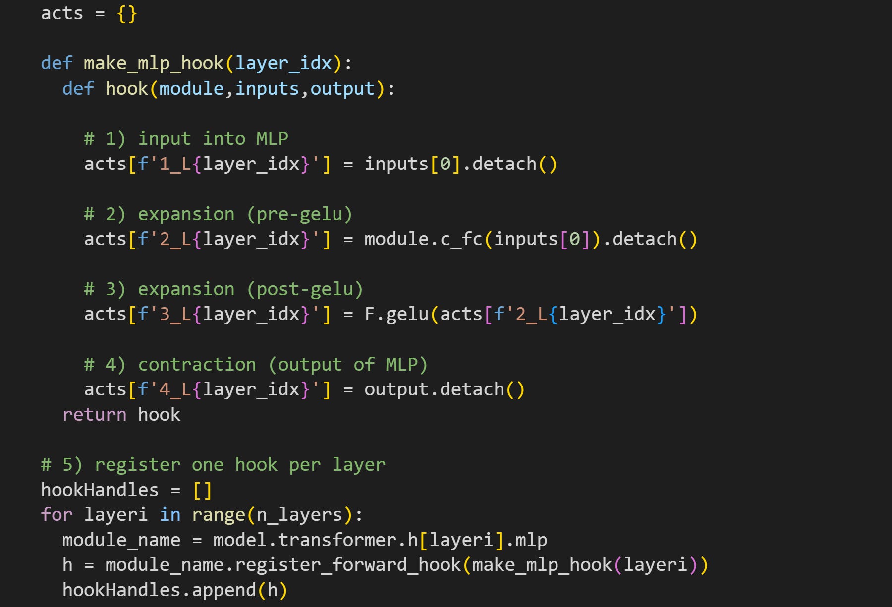
1. First of all, notice that the hook function is implanted into the base MLP layer (comment #5). The line of code underneath comment #1 grabs the input into MLP, before any calculations have been performed. The dimensionality here matches that of the embeddings vectors (1024 for GPT2-medium).

2. Here I get the data from the expansion, before GELU is applied. I do that by pushing the inputs through the c_fc() layer (fc = fully connected). The dimensionality here is 4096 = 1024x4.
   The way I’ve written the code means that the model calls the c_fc layer twice: Once here in the hook function, and then again when the model finishes the hook function and continues the forward pass. Because we’re working with a small amount of text in this demo, that redundancy adds maybe a few milliseconds. But it is an inefficiency to be aware of. You could avoid this redundancy by having two hook functions — one for the main MLP block and one attached to the mlp.c_fc layer — that would eliminate the redundant calculation at the expense of uglier code ¯\_(ツ)_/¯

3. The same data as in #2 but after the GELU nonlinearity. I actually could get these data as the input into c_proj, but I wanted to show you that we can equivalently apply the GELU function to the expansion activations.

4. Finally, the output of the MLP subblock. That is after the contraction, meaning the dimensionality matches that of the token embeddings.

5. Implant all the hooks into the main MLP layer. I’m not manipulating any activations, so the hooks could technically stay in place for the rest of the demo, but I will remove them before Demo 2.

Now we’re ready for text and tokens. In previous posts, I showed that if you call the tokenizer object rather than its encode() method, you get a dictionary that includes an attention_mask. Now in this post, I want to show you how you can use that mask.

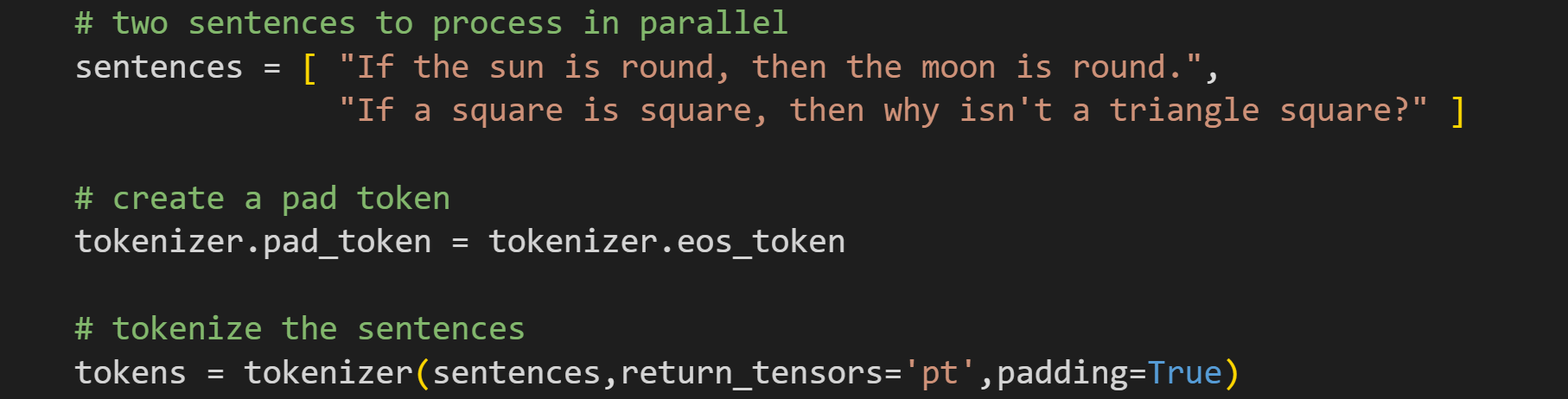
Ahem, I never claimed that these texts would be logical. But the point is that there are two texts, whereas the previous posts had only one. Processing text sequences in a batch is great for many reasons, including computational efficiency and coding simplicity (there are other benefits during training such as batch regularization), but it means that some text sequences might be longer than others. That’s where the attention_mask comes into play.

Below are the input_ids and attention_mask keys in the tokens dictionary.

The first sentence has two repeated tokens at the end — 50256. Those are called “pad tokens,” and the GPT model learns to ignore them. And the attention mask has two zeros at the end; that tells us which tokens are valid and which should be ignored.

How many tokens does the model need to pad? The tokenizer will calculate which sequence in the batch is the longest, and then pad all the other sequences to have the same length. In this example, the second sentence is two tokens longer than the first, and thus, the tokenizer padded the first sequence to match the lengths.

One more bit of housekeeping before pushing the tokens through the model: In the analyses, I want to ignore the MLP activations to the pad tokens and to the first token in each sequence, so I need to know which indices from each sequence to keep.

Figure 6. Screenshot of code to create a list of two lists of indices. I’ll use those indices later to select which activations to keep.

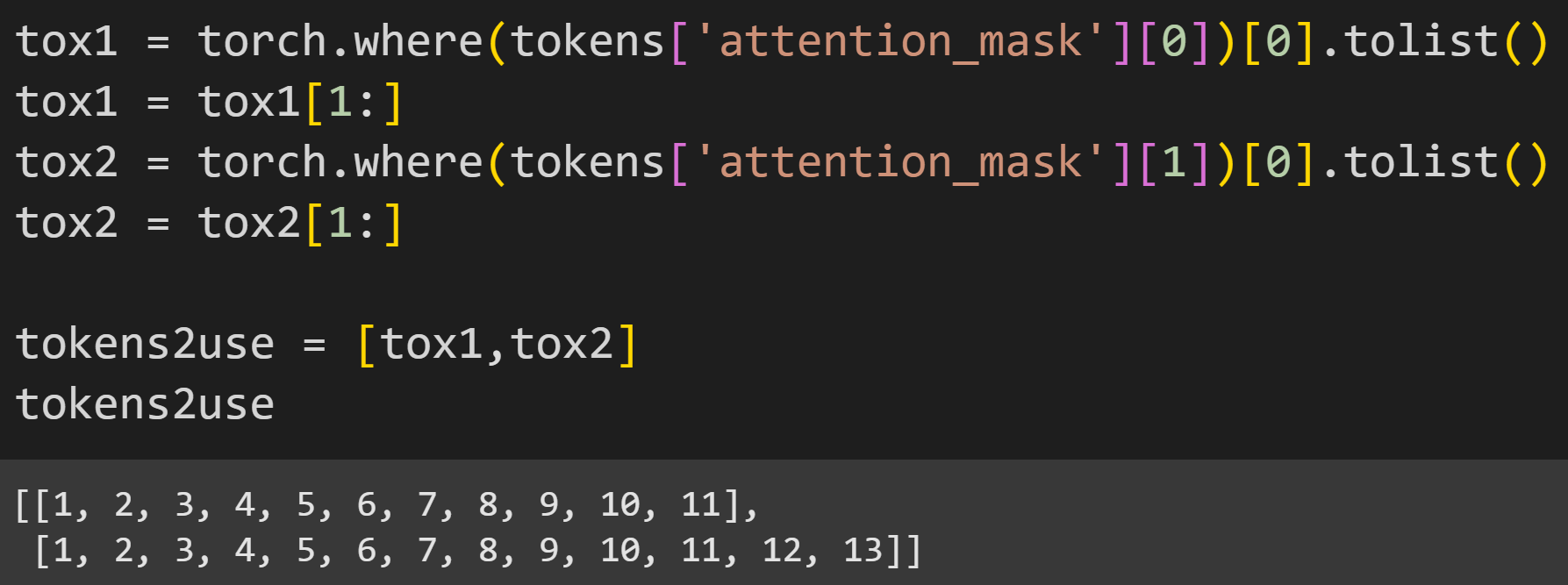
If you’re thinking that this code isn’t scalable because it’s hard-coded to work for exactly two token sequences, then yes, dear reader; you are correct.

Now to run the forward pass to collect the activations, remove the handles, and check the names of the activations.

Figure 7: Screenshot of getting the activations, and printing some of their labels.

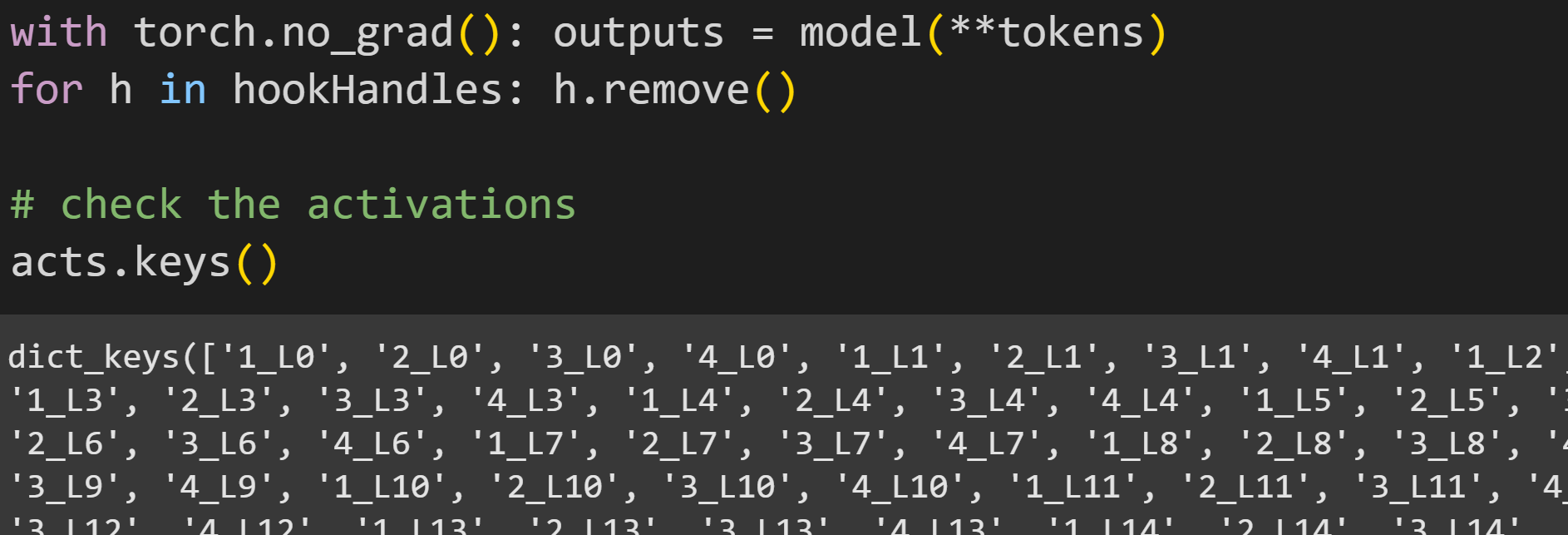
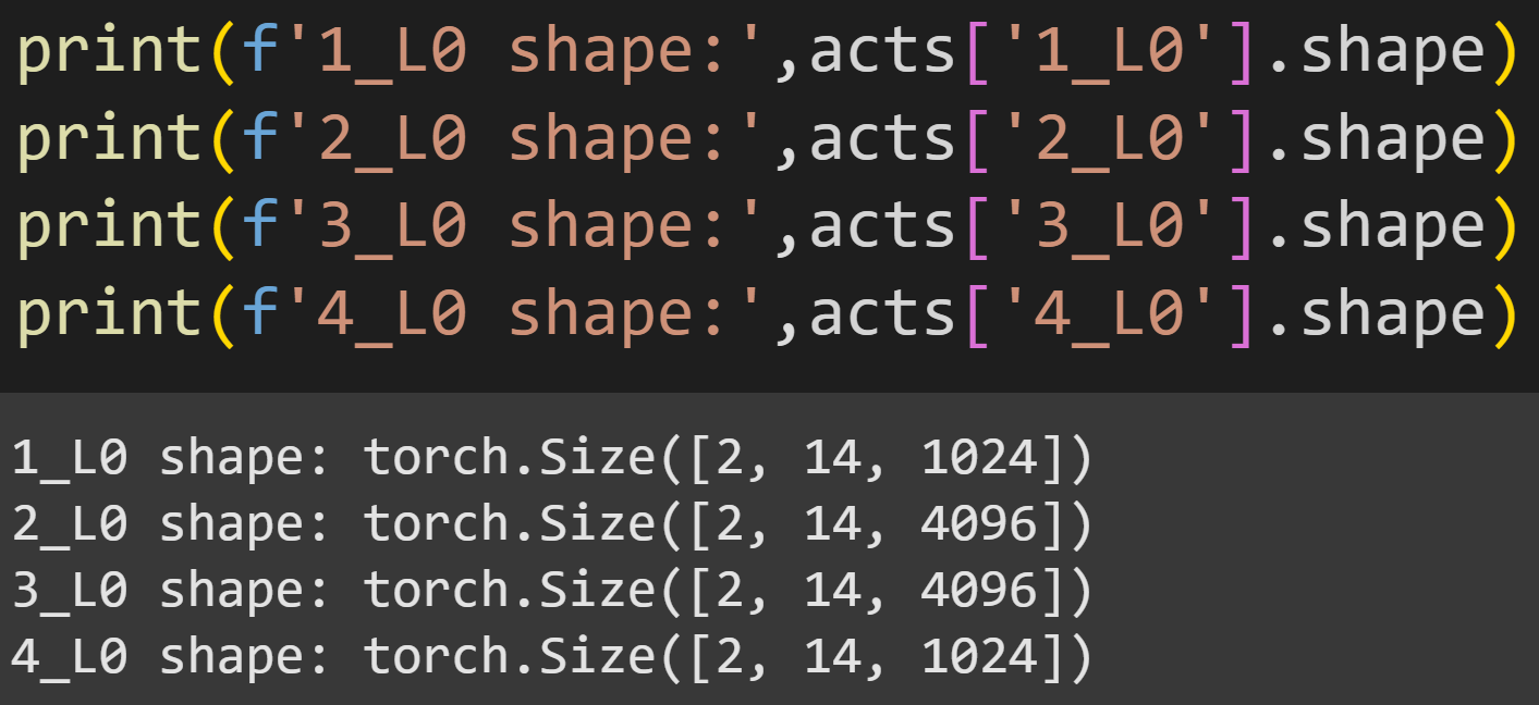
Figure 8 below shows the sizes of the four activations tensors from one layer. All matrices are 2x14, corresponding to two token sequences (the two ridiculous sentences) and 14 tokens (including padding); the final dimension is 1024 for the input and output to the MLP layer, and 4096 for the two expansion activations.

Figure 8: Screenshot showing the sizes of the activations matrices.

Enough preparation, let’s look at some data!

The code below shows how I extract the MLP activations for all valid tokens and from both sentences.

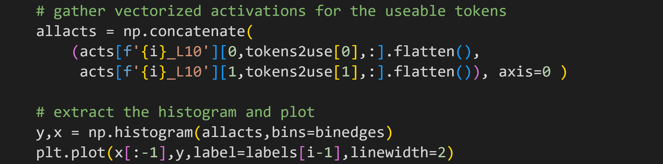
That code goes into a for-loop over the four parts of the MLP block, and produces this fascinating graph:

Figure 9: Distributions of MLP activations. The y-axis was cropped to highlight the broader distributions.

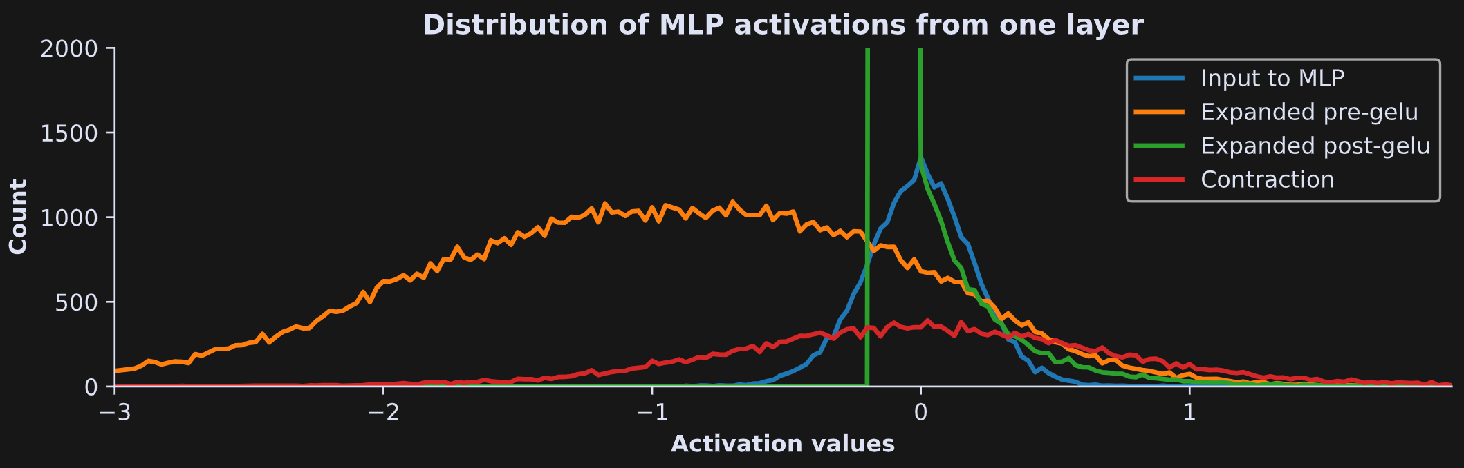
Those are very different distributions, which shows that the different parts of the MLP layer have computationally distinct impacts. Notice, for example, that the MLP input (blue line) has a tight normal distribution around zero, which is then stretched and shifted negative as it gets expanded (orange line). That promotes sparsity because most activations get clipped by the GELU nonlinearity (green line) to facilitate feature extraction and linear separation. Then the contraction calculation widens and normalizes the distribution, which brings it back to the numerical range and distributional characteristics of the embeddings vectors. And in between each of those steps, the activations get transformed and warmed multiple times, analogous to the changes I showed in Demo 0 but in much higher dimensions.

That’s just for one layer… I’m sure you are suuuuper curious what it looks like for all the layers! Just like in the previous post, we can embed the code that extracts those distributions into a for-loop over all the layers in the model, and then visualize the results as images.

Figure 10: images of distributions over the different layers for the four MLP parts.

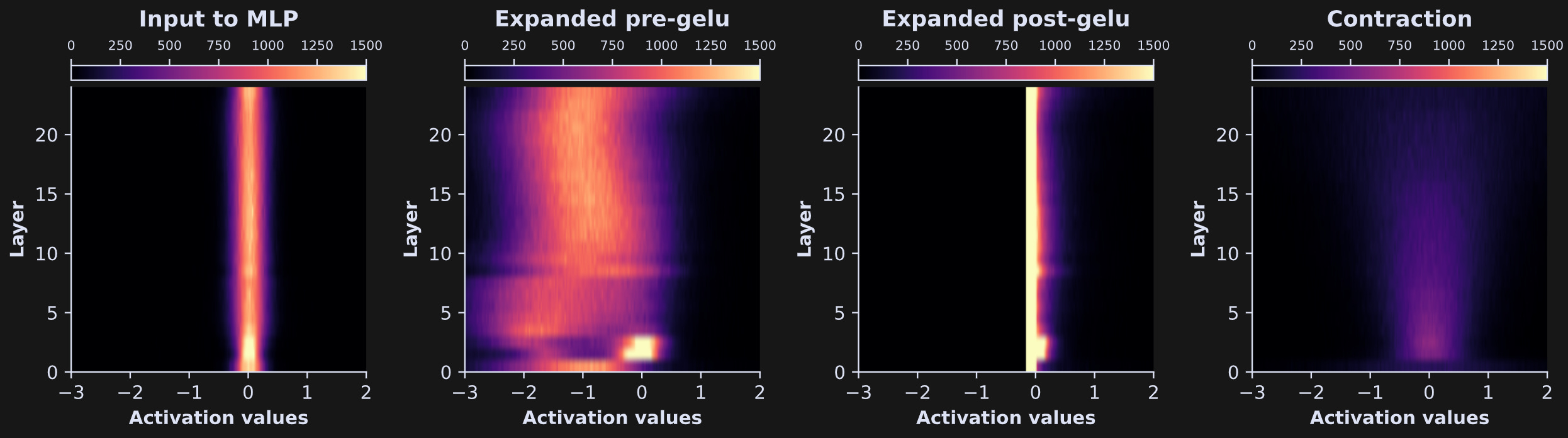
The differences are quite striking, and also quite similar within each MLP part (that is, the laminar differences within each MLP part are small relative to the intra-part differences).

In actual LLM mechanistic interpretability research, investigations like this are the first step. They provide a high-level overview of the model activations, and they would be followed-up by more detailed and insightful experiments. I’ll leave it like this for now, but I do go into more depth in my online course and in other posts here on my Substack.

Demo 2: Imputing high-activation MLP projections

To “impute data” in statistics means to replace some data values with other data values. Imputation is often used in the context of missing or corrupted data; here we will replace a percentage of the most active MLP output projections with the mean of the MLP activations. I’ll start with the tokens.

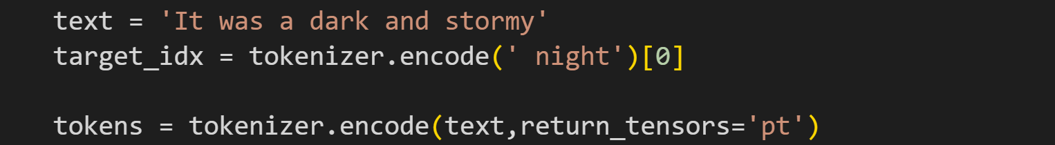
In the experiment, we will manipulate the MLP projections (the output of the MLP sublayer) to determine the impact on the model’s final logit predictions for the token “ night”. Here’s the loop that runs the experiment; as I have often written, I encourage you to try to understand all the code before reading my explanations below.

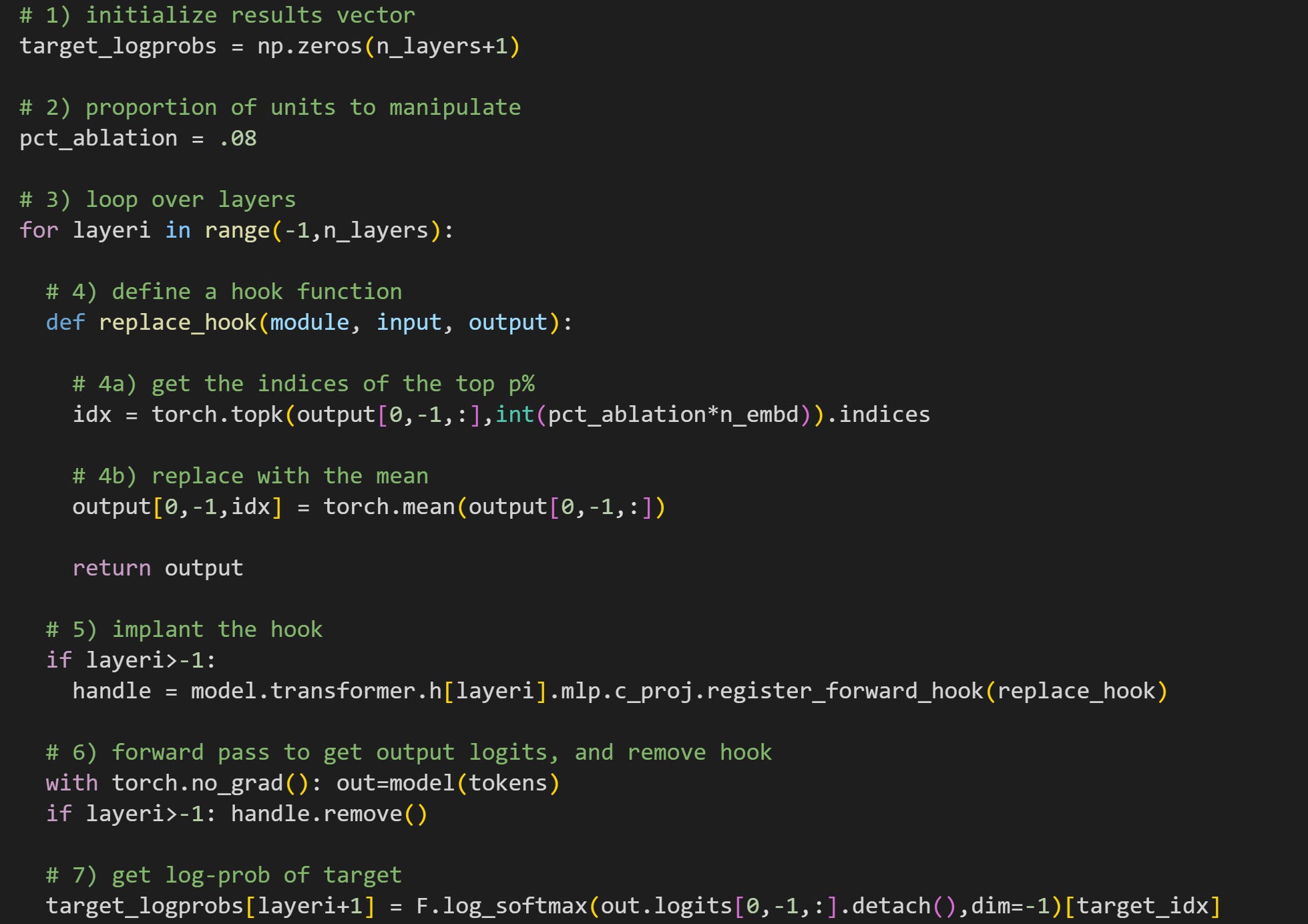
1. The reason to initialize n_layers+1 is that I will use the first element in that results vector for the clean result (no manipulations).

2. Here you can specify how many projection dimensions to impute. I set this parameter to .08 (8%), which is then used in #4a.

3. For-loop over all the layers, plus one. That corresponds to manipulating each transformer block once, plus the clean version of the model without manipulations.

4. This is the hook function. 4a finds the indices of the most active dimensions. The product pct_ablation*n_embd converts proportion into a number of dimensions (e.g., int(.08x1024)=82). 4b replaces the activations at those indices with the average of the MLP outputs. Notice that all of these calculations happen only for the final token in the sequence. It is, of course, possible to manipulate any token in the sequence, but focusing on the final token ensures that we’re not screwing up the model’s ability to incorporate world knowledge and local context before making a prediction about the new token. In other words, this is a small but targeted and precise manipulation.

5. Having the conditional if layeri>-1 is the mechanism that produces a clean model: the hook is only implanted starting at layeri=0.

6. Forward pass and removing the hook. This line also needs the if-conditional, otherwise you’ll get an error when trying to remove a handle that isn’t yet defined.

7. Finally, get the output logits of the final token, log-softmax, and pick out the log-probability value of the target word index (“ night”). The indexing layeri+1 is necessary because I started the looping index at -1.

And here are the results!

Figure 11: Results of the experiment in which the most active MLP projections were replaced by the MLP average. Y-axis is the log-probability of selecting the next token “ night” from the model’s final output logits.

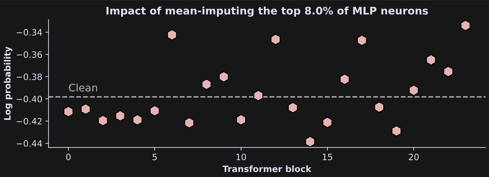
There is no clear pattern of results, in the sense of consistently increasing or decreasing as a function of layer. Instead, it seems that reducing the highest-activated MLP projections added some variability to the final token selection. LLMs are extremely complex systems, and it is not always straightforward to interpret such subtle manipulations.

THE END (of the beginning)

Thank you for joining me on this journey into LLMs! I know there are a bajillion LLM explanations out there; my intention was to make one that is more hands-on, engaging, scientific (in the sense of running experiments and visualizing data), and empowering than other tutorials I’ve seen.

LLMs make for fantastic research topics, both for complex systems analysis and for technical AI safety. If you feel inspired by this post series, then please keep learning (ahem, perhaps using my in-depth course on the topic).

Final note

I write these posts because I love doing it… but also because it’s my job. It’s my work and my source of income. If you would like to support me, please enroll in my online courses, buy my books, or become a paid subscriber here on Substack. Thank you kindly :)

Detailed video walk-through of the code

The 24-minute video below is available to subscribers whose support allows me to continue creating posts for you to read. If you’re one of them, I’m grateful for your contribution!