LLM breakdown 3/6: Embeddings

Embeddings vectors are the key to the complexities and subtleties of language.

About this 6-part series

Welcome to Post #3 of this series!

The goal of this series is to demonstrate how LLMs work by analyzing their internal mechanisms (weights and activations) using machine learning.

Part 1 was about transforming text into numbers (tokenization) and part 2 was about transforming the final model outputs (logits) back into text. Now you’re ready to start learning about the magic inside the box.

Part 3 (this post) is about embeddings vectors. Embeddings vectors are high-dimensional representations of tokens. THEY ARE VERY IMPORTANT. Really. LLMs don’t work with text, and they don’t work with tokens. They work with embeddings vectors. The entire purpose of transformers and the attention algorithm is to tweak the embeddings vectors as they pass through the model.

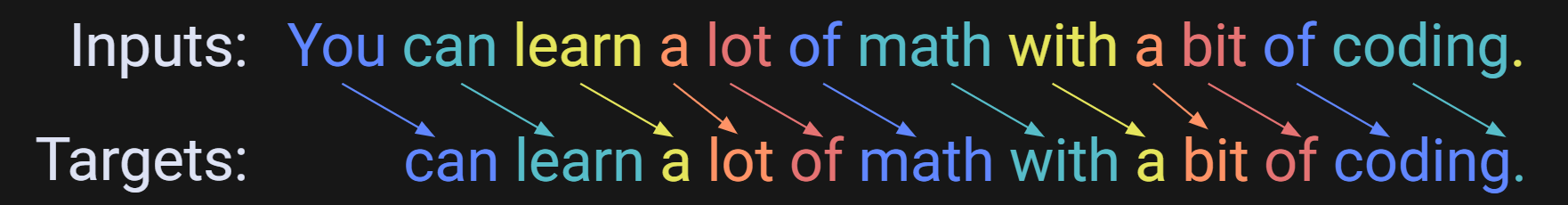
Use the code! My motto is “you can learn a lot of math with a bit of code.” I encourage you to use the Python notebook that accompanies this post. The code is available on my GitHub. In addition to recreating the key analyses in this post, you can use the code to continue exploring and experimenting.

What are embeddings vectors?

You know about tokenization: converting a character string (technically, a byte sequence, but it’s easier to talk about characters and subwords) into an integer. Embeddings vectors are another way to represent tokens using numbers. Whereas tokenization maps one token to one integer, embeddings map one token to hundreds or thousands of floating-point numbers in a vector.

Why is it better to represent text using a dense vector instead one integer? Well, with embeddings, we don’t actually want to compress the text; we want to expand it in a way that allows for rich, contextual information to be associated with each word. For example, the GPT2 tokens for “ apple” and “ pear” are 17180 and 25286. Apples and pears are closely related to each other semantically, and yet those two integers have no way to express that relationship. Furthermore, if we’re prompting ChatGPT about apple pie vs. apple juice, we want ChatGPT to understand that it’s the same fruit but used in different ways. Again, the number 17180 doesn’t allow for subtle context-based modulations.

Embeddings vectors, unlike token indices, endow words with rich semantic information that can be adjusted according to the context of the text.

I’ll introduce embeddings spaces in a very concrete way — then in a more abstract though accurate way.

Consider the 2D axis in Figure 1. It’s a 2D embeddings space where the two axes are Size and Friendliness. We can represent animals in this space according to how big they are (x-axis) and how friendly they are (y-axis).

Figure 1: Illustration of a 2D embeddings space with five embeddings vectors shown.

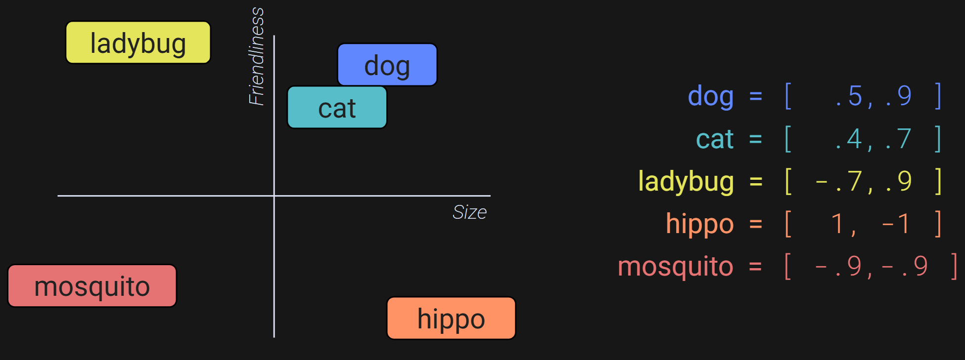
The numbers on the right are (x,y) coordinates that indicate the position of each animal in this space. Those are the embeddings vectors for the words. You can see how the embeddings vectors capture information about the relations among the animals (e.g., dogs and cats are similar size and friendliness; ladybugs are only a little bit bigger than mosquitos but are much friendlier), compared to a tokenization scheme of dog=1, cat=2, ladybug=3, etc.

Furthermore, the embeddings vectors are not static; they can change. Let’s say we’re talking to ChatGPT about how our neighbor’s cat hisses and scratches; ChatGPT can subtract from the Friendliness dimension without changing the Size dimension. So, the LLM can use context (previous tokens) to adjust the embeddings vector for the word cat to [.4,.6].

I hope Figure 1 and my description highlight the advantages of dense embeddings over single integers. But it’s much more complicated — and much less interpretable — in real language models, for several reasons:

1. Token embeddings are very high-dimensional. Even a “small” LLM might have an embeddings dimensionality in the thousands. The GPT2-small LLM has an embeddings dimensionality of 768 and the XL version has 1600 dimensions.

2. Actual embeddings dimensions are not human-interpretable. There is no “size” axis and “friendliness” axis. People have tried to define interpretable axes inside embeddings spaces, but it doesn’t really work and the conclusions are way overblown. Perhaps you’ve heard about the “king-man+woman = queen” phenomenon in embeddings spaces. I’m going to write another post just about that (this sentence will be replaced with a link when I do!), but the short version is that it’s mostly bullshit. There is a very small number of hand-picked examples where vector arithmetic translates to human-interpretable analogical reasoning, but it’s just not a real phenomenon that generalizes to many examples.

3. The embeddings vectors change as they pass through the model. At each step inside the model, an adjustment to the vector is calculated and added, like with the analogy of reducing the Friendliness dimension in the neighbor’s antisocial cat. This means that the effort you put into making a human-interpretable embeddings vector won’t necessarily apply after even the first of many transformations that the vectors undergo.

4. The embeddings vectors are different for different language models. For example, all models in the GPT2 family have exactly the same tokenizer, but they all have completely different embeddings vectors. Even if you create two LLMs of the same size and train them from scratch on exactly the same text data, they will have different embeddings vectors simply because of the different random initializations.

None of these four points are limitations — quite the oppose. But they are reasons why individual embeddings vectors are not human-interpretable. On the other hand, relations across embeddings vectors can be interpreted, which I’ll demonstrate in demo 2.

Code demo 1: Import and visualize embeddings vectors

If you study natural language processing, you’ll learn about embeddings matrices like Word2Vec and GloVe. Those embeddings were important in the development of computational linguistics and language models, but they aren’t used in modern LLMs. Therefore, I’m only going to focus on embeddings vectors that are built into LLMs like OpenAI’s GPT2.

To get GPT2’s embeddings vectors, we need to import the entire model. The embeddings are in a layer called wte — word token embeddings. (Friendly reminder: Only the essential code snippets are shown in the post; you can get the full code file on my GitHub).

Figure 2: Isolating the matrix of embeddings vectors.

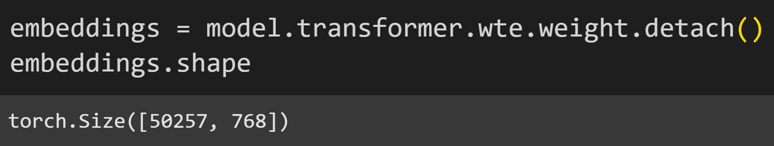
That first size (50,257) should be familiar to you after having gone through the previous post: It’s the number of tokens in GPT2’s vocabulary. The second size (768) is the embeddings dimensionality of GPT2-small. The dimensionality is fixed within a particular model, but varies across different models. For example, the “XL” version of GPT2 has an embeddings dimensionality of 1600. GPT3 models have embeddings dimensionalities up to 12,000. The dimensionalities of the newest commercial models like GPT5 are not public, but are probably several tens of thousands.

Not even the fabulously dressed Leonardo Davinci could visualize a 768-dimensional coordinate system, so instead, embeddings vectors can be plotted with the dimension index on the x-axis and the value (that is, the coordinate) in each dimension on the y-axis. The left-side panel of the figure below shows the embeddings vectors for two words.

Figure 3: Visualization of embeddings vectors for two words (left panel). Each x-axis value corresponds to a dimension (thinking back to Figure 1, for example, the x-axis would have two values), and the the y-axis shows the coordinate in that dimension. The right panel shows the relationship between the embeddings for two words.

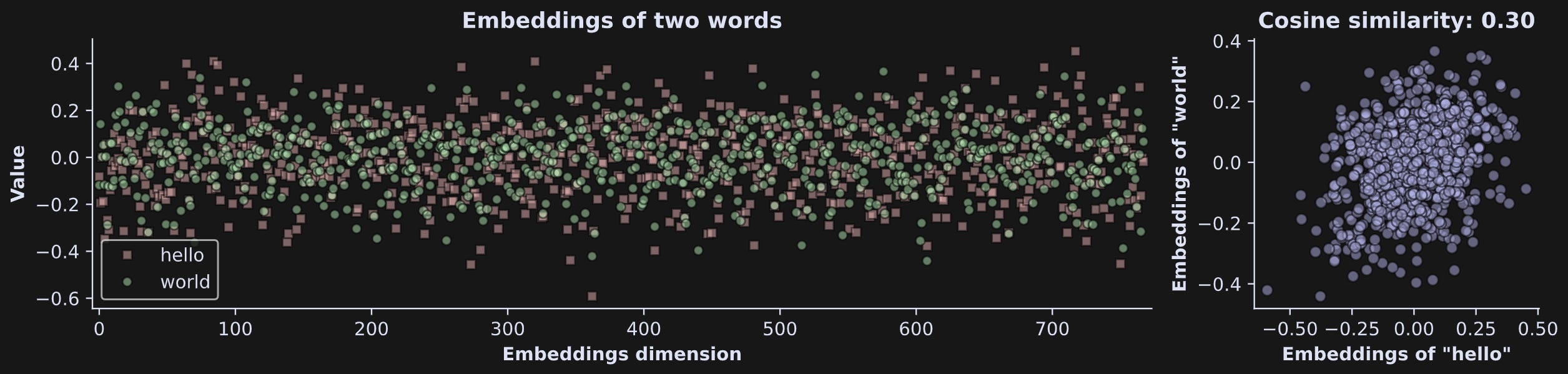
“hello” and “world” are often used together in language and coding, so we might expect a positive relationship between them. Indeed, their cosine similarity is .30. Cosine similarity is a statistical measure of the relationship between two variables, and varies between -1 and +1. A value of .3 indicates a modest relationship¹. Curiously, the cosine similarity between “ hello” and “ world” (with preceding spaces) is lower (.21).

If you’re following along with the online code (which I super-duper-really-a-lot recommend!) then take a minute to explore some embeddings pairs. For example, do “apple” and “pear” have higher cosine similarity compared to “apple” and “spaceship”?

The entire embeddings matrix can be visualized using a heatmap. In the image below, each column is a token and each row is an embeddings dimension, and each pixel in the image corresponds to the coordinate value of one token in one embeddings dimension. The color corresponds to that value, same as the y-axis in the previous figure.

Figure 4: The color of each pixel in this image indicates the value of each embeddings dimension (y-axis) for each token in GPT2 (x-axis).

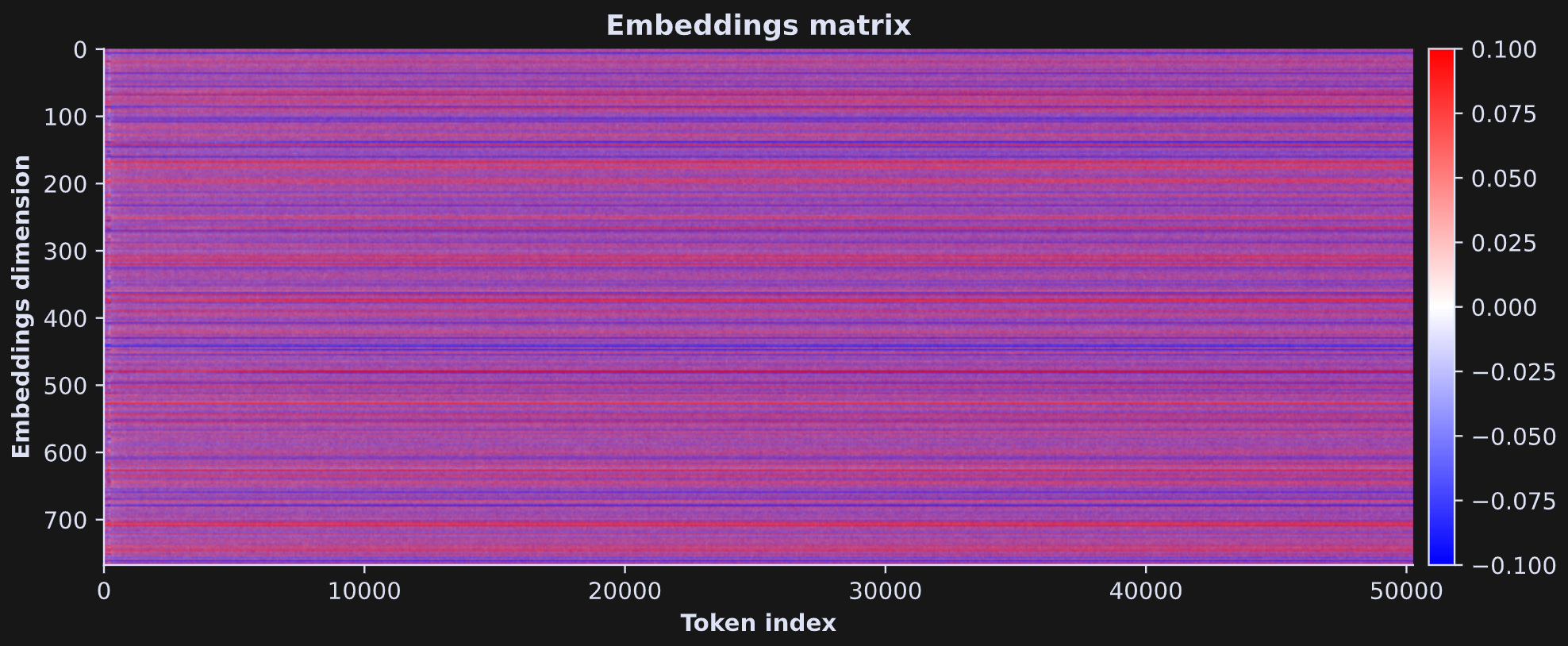
The horizontal stripes are quite striking. Some dimensions have positive offsets for all tokens (red stripes) while other dimensions have negative offsets for all tokens (blue stripes).

The previous two figures show the initial embeddings; how they look at the very start of the LLM. But embeddings vectors are not static. They are dynamic. They change throughout the language model. In fact, each embeddings vector changes four times per transformer block (two normalizations, one attention adjustment, and one MLP adjustment). Understanding those adjustments is the goal of the next several posts.

But don’t get me wrong: It’s not that embeddings vectors are completely random and totally uninterpretable — embeddings vectors for semantically similar words have are related to each other, while you’ll see in Demo 2 later in this post.

Where do embeddings vectors come from?

Embeddings vectors are part of the LLM, and as such, they are trained through next-token prediction alongside the rest of the model. In this sense, the embeddings vectors are not privileged or special; they are parameters to optimize just like every other parameter in the LLM. (Non-LLM embeddings like Word2Vec are trained in a different way, but I won’t discuss that here.)

When a new LLM is created, all the weights in the model, including the embeddings vectors, are initialized to random numbers. Then the model is given text and asked to predict each token based on the previous tokens.

Figure 5: Models try to predict the next token in a sequence.

After each prediction, the weights are adjusted to increase the model’s next-token prediction accuracy. That’s done through a procedure called gradient descent. After training on billions to trillions of tokens, the model weights converge on values that help the model make more accurate predictions.

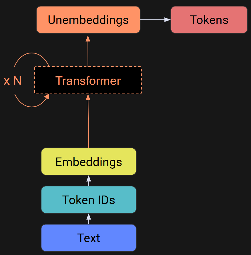
Lifecycle of embeddings vectors through the LLM

Figure 6 below shows a graphical overview of an LLM. Text gets tokenized, and the token indices pick out columns of the embeddings matrix, which are the embeddings vector for each token. Those embeddings vectors get passed through the rest of the internals of the LLMs — mainly the “transformer block,” which has two subparts (attention and MLP) and several normalizations. Each of those steps involves calculating small adjustments to the vectors, rotating and stretching them.

Figure 6: Overview of an LLM. The entire purpose of an LLM is to transform an embeddings vector from the current token to a prediction about the next token.

At the beginning of the model, each embeddings vector points to the token from whence it came, but by the end of the transformer block sequence, the embeddings vector no longer points to the current token, but instead, it points to a predicted next token. The vectors are constantly getting pushed and pulled and prodded, and that’s why you shouldn’t worry too much about interpreting the initial embeddings vectors.

Code demo 2: Dimension-reducing embeddings vectors

The embeddings dimensionality of GPT2-small is 768, which is a challenge to visualize. But we can visualize a 2D projected version of that high-dimensional space. Any low-dimensional projection is likely to lose a lot of information, but hopefully the projection preserves key information that facilitates understanding.

I’ll use a dimension-reduction technique called T-SNE. The idea of this method is to create a lower-dimensional projection of high-dimensional data that preserves the distances between individual data points.

I took the first 100 embeddings vectors, corresponding to the first 100 tokens, and applied T-SNE. The scatter plot below shows their projections along with the label of each token.

Figure 7: The 768-dimensional embeddings vectors for the first 100 tokens were projected down to two dimensions. Each little circle is a token and its corresponding text is printed above. The clustering naturally emerged.

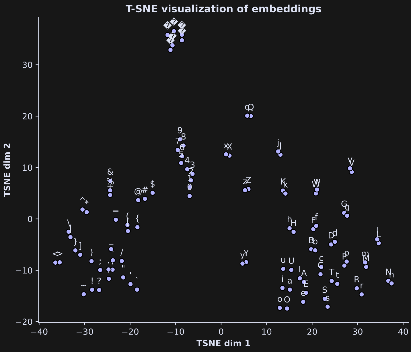
It’s very cool to look at: The digits cluster into a line; lower-case and upper-case letters are close to each other; punctuation marks, math symbols, and brackets form a group. The question-mark-diamond shapes at the top-left are other formatting characters like new-line, tab, and carriage-return.

Code demo 3: Manipulating embeddings vectors

I’m a scientist. Well, not by paycheck anymore, but still: You can take the scientist out of science, but you can’t take the science out of a scientist. I like to learn by running experiments. So let’s run some experiments on embeddings vectors.

We’re going to work with the following text:

The capital of Germany is

Of course you know that the next word is likely to be “Berlin.” It could be other words, like “the” as in, “the city called Berlin.” But the next word certainly isn’t “Paris,” unless we change “Germany” to “France.”

And that’s exactly what we’re going to do. We will replace the embeddings vector for “ Germany” with the vector for “ France”, and see what happens to the model output logits for the target words “ Berlin” and “ Paris”.

(btw, I’m writing “we” here because although I wrote this post and the code, I want you to run the code and be an active participant.)

Let’s build up this experiment one piece at a time. Start with the text to process.

# the main text
text = 'The capital of Germany is'

# source and target tokens
source = ' Germany'
target = ' Berlin'
distractor_source = ' France'
distractor_target = ' Paris'

btw, if this were a real experiment, it would be good to check that the source and target words really are single-token words, although that is the case here (for multitoken words, you use only the final token because it absorbs the context from the previous tokens).

Next, tokenize these texts and find the position of the token we’ll replace.

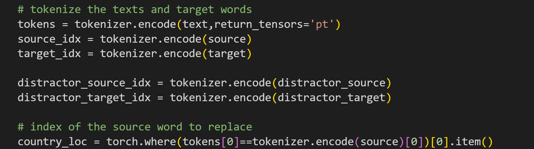
We’re almost ready to run the experiment. The idea is to process the text and get the output logits for “ Berlin” and “ Paris”, like this:

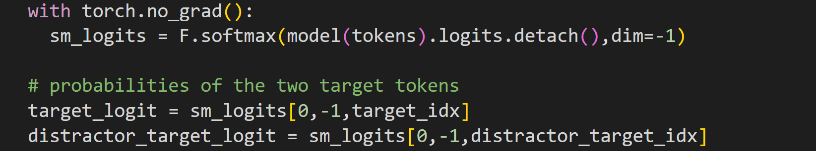
Notice that I’m running the model, extracting the logits, and converting to softmax all in the same line of code. That’s fine here because the token probabilities are all we care about in this experiment. Just be mindful that this means we no longer have access to the raw logits.

The probabilities from the final token (which are the model’s predictions for what comes next) are 5.27% for “ Berlin” and 0.13% for “ Paris”. The model doesn’t overwhelmingly favor “ Berlin” as the next token, but it clearly thinks that “ Berlin” is more likely than “ Paris”.

Now for the manipulation. Here’s the code for the hook function. As in my previous posts, the numbers in the comments correspond to explanations below.

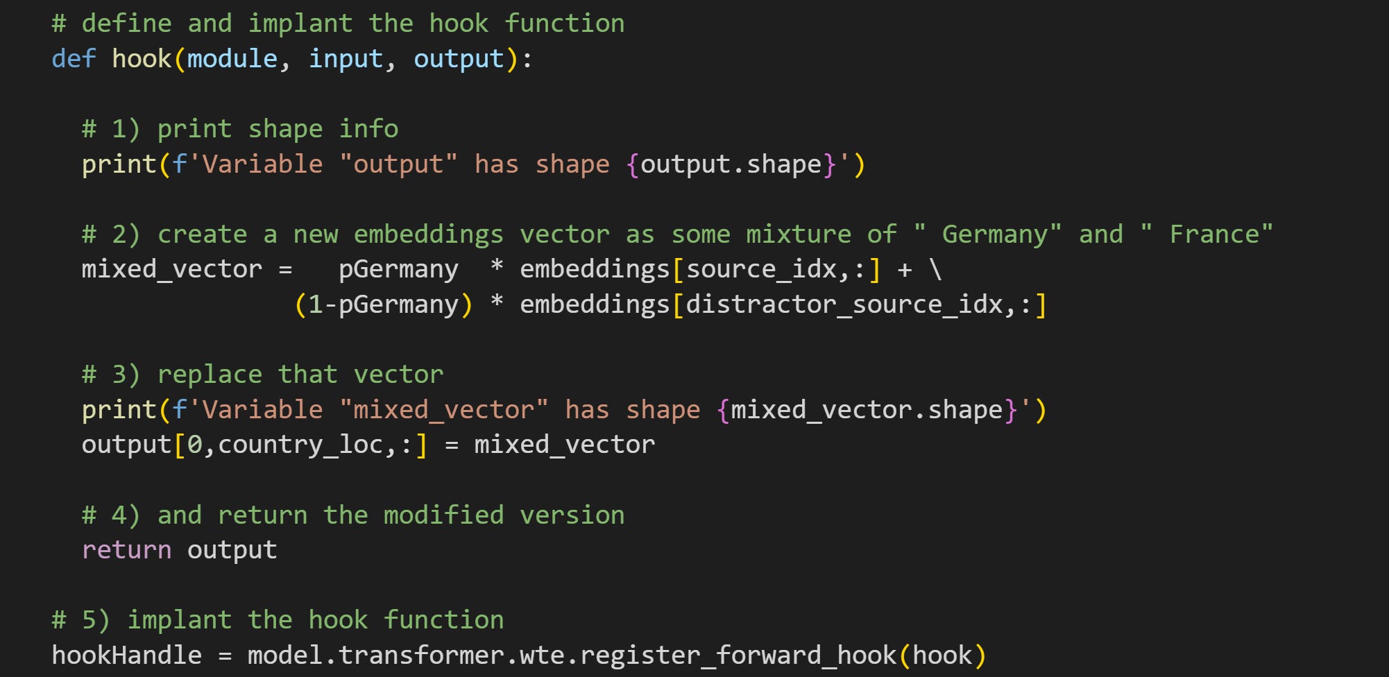
1. When the hook function gets called during a forward pass (when you push tokens through the model), it will print out the size of the output tensor. Remember from the previous post that this variable is the output of the implanted layer, in this case, the wte layer that contains the embeddings matrix. Printing information like this is a fantastic way to help you develop code and find and fix bugs. But you’ll want to remove it (or comment it) when running real experiments, because it slows the calculations and crowds up your Python window.

2. Here’s the key line that creates the manipulation. The code adds together two embeddings vectors, one for “ Germany” and one for “ France”. They get proportionally mixed by the variable pGermany. Consider that when pGermany=0, the mixed_vector is completely replaced with the embeddings vector for “ France”. And when when pGermany=.5, then mixed_vector is 50% Germany and 50% France.

3. That new mixed vector replaces the position of the country in the original text. This is how the manipulation is implemented. I’ve also included code to print out the sizes. And again, this is the kind of code you should include when developing your code, but then comment out after ensuring accuracy.

4. You can create hook functions without a return line, but then it won’t actually do any manipulations. Non-outputting hook functions are used to get data from the model. You’ll see that in the next few posts. But with the return line, the output of the hook function overwrites the output of the model layer.

5. Implant the hook function into the wte layer. As I wrote in the previous post, the output of the function is a handle (like a pointer) to the function in the model. You can use that handle to remove the hook, which is helpful when developing your code to remove buggy hooks, or if the experiment involves replacing hook functions to perform different manipulations.

The first thing to do after creating and implanting the hook is to set pGermany=1 and then re-run the previous code block. We should get identical softmax-probability outputs as before, which provides a good check that our hook function is correct.

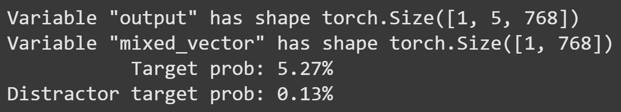
Figure 8: Screenshot of Python output with the hook implanted and pGermany=1.

The forward pass of the model called the hook function, which printed the size information. Importantly, the probabilities of the two tokens are the same as before. These outputs indicate that our hook function is working as expected.

Next I’ll set pGermany=0 and run the code again.

Figure 9: Same as Figure 8 but pGermany=0.

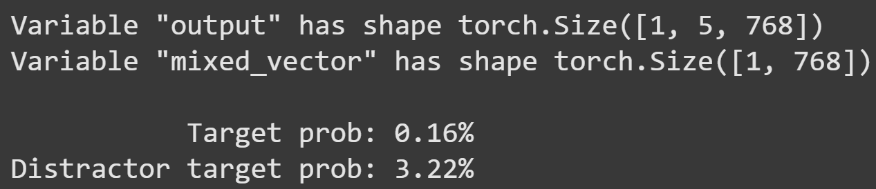
When the embeddings vector for “ France” replaces that of “ Germany”, the model prefers “ Paris” 20x more than “ Berlin”.

Pretty interesting, wouldn’t you say? No? You disagree, and you’d like to know what happens when we mix the two vectors? Well, dear reader, let’s do that experiment.

What we’ll do now is vary the pGermany variable between 0 and 1 in 17 steps. I won’t show the code here in the post because it’s nearly identical to the code block above, just in a for-loop over different values of pGermany. Of course, it’s in the online code file and I encourage you to follow along there. (Running that experiment prints out 34 lines of tensor sizes, which is aesthetically displeasing and redundant, and which is why you should remove the printing code from the hook function.)

Here are the results!

Figure 10: Results of the experiment show that as we smoothly change the mixture of embeddings vectors, the probability of the model selecting “ Berlin” also smoothly changes.

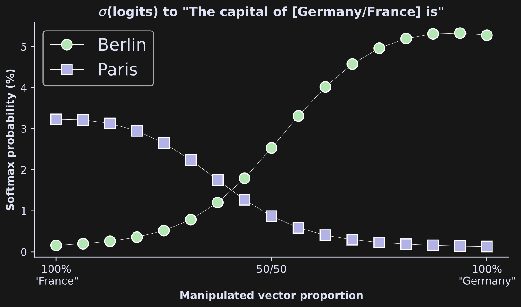
The x-axis shows the mixture proportions and the y-axis shows the softmax-probability of the two target words. The effect is beautiful: As we manipulate the embeddings from one country to another, the model smoothly switches its prediction about the capital city. It’s also interesting that at the 50/50 mark, the model still prefers Berlin over Paris, and that the preference for “Berlin” with “Germany” is higher than the preference for “Paris” with “France” (no comment).

Conclusions about embeddings vectors

Embeddings vectors are the shit. Da bomb. Literally the foundation of all chatbots. Those vectors start off as just merely a set of numbers in a look-up-table, but they get tweaked, twisted, transformed, and turned, as they pass through the model. All of that magic happens inside the transformer block, and that’s what you will learn about starting in the next post.

Thank you for trusting me with your LLM education

Congrats on being half-way through this series! I hope you’re finding it a worthwhile use of your time. If you’re ready to dive much deeper into LLMs, check out my full-length course on using machine-learning to understand LLMs.

If you’d like to learn more from me — and support me at the same time — then please consider enrolling in some of my longer video-based courses, buying my books, becoming a paid Substack subscriber, or just sharing my work with your friends (“like and subscribe” yada yada). Much appreciated :D

1. It turns out that nearly all embeddings vectors have positive similarity to all other vectors. The embeddings vectors are distributed in a “hyper-conoid” in the embeddings space instead of being uniformly distributed. That’s just one of the myriad fascinating nuances of LLMs that short posts like this doesn’t really allow for.