
Two-variable dependence part 1: Covariance
Learn the theory and code of the most important and foundational statistical measure of linear relationships.

About this three-part series
I wrote this post series because many people are confused about how covariance and mutual information are related to each other, and when to use which one. It’s an understandable confusion: both covariance and mutual information measure the relationship between two variables. But they really are different, and have different assumptions, provide different insights, and are used in different applications.
In Part 1 (what you’re reading now) you will learn about covariance, which is a simple yet powerful way to measure the linear relationship between two variables. Covariance is a workhorse of data science, and is the basis for analyses such as correlation, principal components analysis, linear classifiers, signal processing, multidimensional approximations, regression, and a lot more.
In Part 2 you will learn about mutual information, which is conceptually similar to covariance but is based on a different equation and therefore has different nuances and challenges. But it does measure nonlinear relationships, which is a major advantage.
And finally, in Part 3 you’ll see a direct comparison between the linear (covariance) and nonlinear (mutual information) approaches.
Follow along using the online code
Only the essential code snippets are shown in this post; the full code file to reproduce, extend, and adapt the analyses are in the code file on my GitHub. It’s one Python notebook file for the entire post series, so this post covers only the first 1/3 of the notebook file.
The video below will help you get started with importing the Python notebook from into Google Colab.
What are “bivariate linear relationships”?
Well, first of all, a “bivariate linear relationship” is a really nerdy thing to say. It’s probably not the most romantic way to express your relationship intentions to your crush (unless your crush is also a stats-nerd).
But more seriously: Bivariate means between two variables, and linear means the relationship can be captured using a straight line. The figure below shows some examples of bivariate linear and nonlinear relationships, and their covariances.
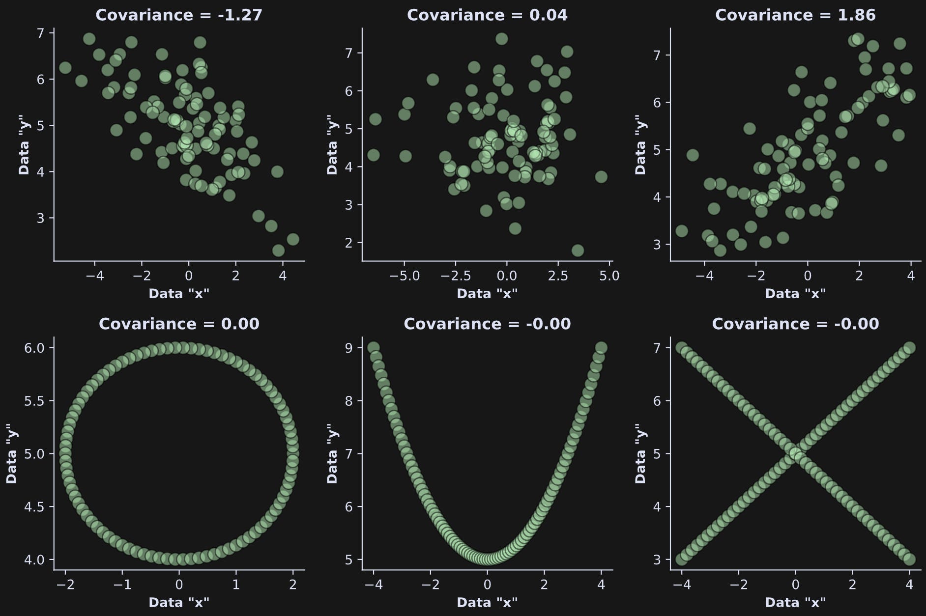
Covariance — the topic of this post — is a linear measure, and therefore, cannot reveal nonlinear relationships. For that, you need mutual information, which is the topic of Post 2 in this series.
What is covariance?
In this section, I will show you the formula for covariance and explain details about how to interpret it, and then the next several sections will help you build intuition through Python code demos with examples and visualizations.
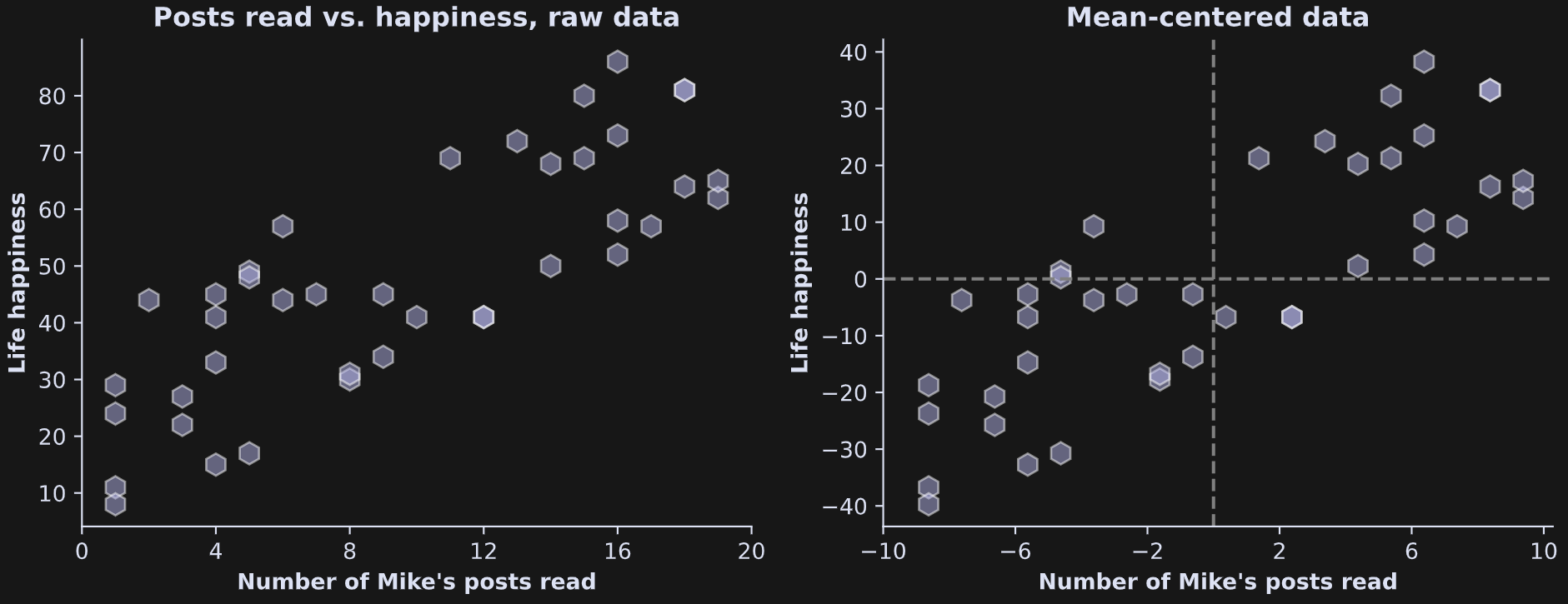
Let’s start with a concrete example to help work through the equation. Imagine I surveyed some of my readers on Substack and got two data points from each person: the number of my Substack posts they’ve read, and their self-reported life happiness. The left panel in the figure below shows the raw data, and the right panel shows exactly the same data but mean-centered. You’ll understand why the data are mean-centered in a bit.
Clearly, the conclusion here is that if you want to have a happy life, you need to read more of my Substack posts 😌
OK ok, just kidding. These are fake data that I simulated for this figure (in fact, you can create your own fake data using the online code).
And even if these were real data, covariance is non-causal. That is, covariance does not establish or even imply a causal direction; covariance does establish that two variables are statistically related, but whether that relationship is causal or even direct needs to be established by an experimental manipulation.
Negative covariance indicates that one variable goes down when the other goes up; positive covariance indicates that both variables go up and down together; zero covariance indicates that the variables have no linear relationship. The covariance in Figure 1 is positive.
The equation below is the formula for covariance; x and y are the two variables (let’s set x = number of posts read and y = life happiness), x-bar and y-bar (that is, the x with a bar on top) are the averages of each variable, and N is the sample size.

I have several comments and nuances about this formula:
The variables must be mean-centered before calculating the covariance. Mean-centering ensures that the sign of the covariance matches the relationship between the variables. Imagine leaving out that step: Posts-read and life-happiness are both positive, and so even a negative relationship between posts-read and happiness would still yield a positive value of C. On the other hand, when variables are mean-centered, people who read below the average number of posts but have above average happiness will contribute a negative number to the summation.
The covariance is scaled by N-1. The reason for scaling is to prevent the covariance from trivially increasing with sample size (in other words, scaling changes the sum to an average). You might have initially expected to scale by 2(N-1) because there are two variables and two sample means. But the "statistical atom" here is a pair of data points, not an individual data point, and there are N pairs.
There is only one N term; there aren’t separate N terms for each variable. Covariance requires a pair of variables measured from the same subjects. In this example, you can examine covariance in posts-read and life-happiness in the same people, but you cannot examine covariance in posts-read in one group with life-happiness in a separate group.
The unit of covariance is the product of the units of the individual variables. If both variables have the same units, then the covariance units might be interpretable (for example, time series signals, which could have covariance units of squared volts). In many cases, the units are not easily interpretable. In our example here, the covariance unit is “count-happiness,” which has no real interpretation (if you think you can interpret it, you’re probability thinking of happiness divided by count, for example from a regression, but that’s not the units of covariance). For many applications of covariance, the units are not interpretable and are therefore ignored.
Covariance is commutative (commutative is the property in math that a*b=b*a), meaning that the covariance between posts-read and happiness is the same as the covariance between happiness and posts-read. This symmetry is the reason why you cannot infer causality from a covariance (or correlation) analysis.
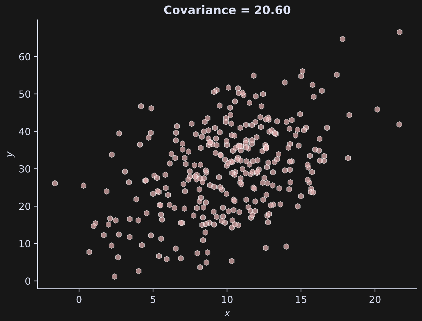
Demo 1: Covariance in simulated data
I’m a big fan of learning data science through simulated data: You can create as much data as you want, specify the sample size and data characteristics, explore the impact of outliers, and so on. On the other hand, there’s no substitute for real data; I’ll use real datasets in Part 3.
I admit that I considered writing the rest of this post using posts-read and life-happiness, but it started to feel a bit awkward. So I’ll switch to using meaningless and unitless variables.
A simple way to create two linearly related variables is as random numbers, with one variable summed into the other. It looks like this:
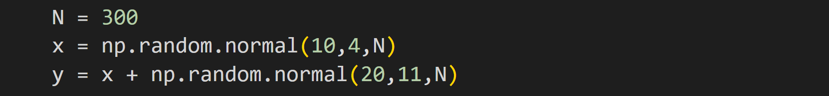
That method does not allow for controlling the exact strength of the relationship, but it is fast and easy. (I explain how to control the strength of the linear relationship in this post.)
Now to calculate covariance. The code below is a direct translation of the math formula I showed earlier.
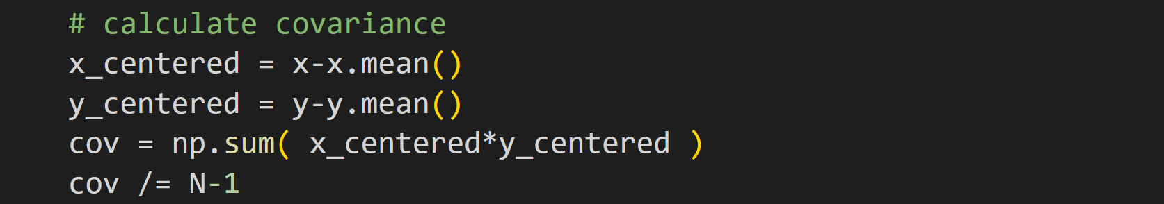
Translating math directly into code is a fantastic way to learn data science, but in practice it’s often more convenient to use functions that come with libraries.

Notice how I index the variable cov_np; the np.cov() function returns a matrix of covariance values, which is useful for multivariable datasets. In this case, we have only two variables and so we need only one off-diagonal element.
Here’s what the data look like:
Covariance and correlation
One awkward aspect of covariance is its dependence on the scale of the data. That is, there is a relationship between height and weight (taller people tend to weigh more), but the covariance value depends on whether the data have units of kilograms vs. pounds, or feet vs. centimeters. That’s demonstrated in the code file.
That’s where the correlation comes into play. The correlation coefficient is simply the covariance divided by the variances of the variables. That normalization factor eliminates the scaling effects by standardizing both variables. The first equation below is covariance (repeated for comparison), and the second is correlation.
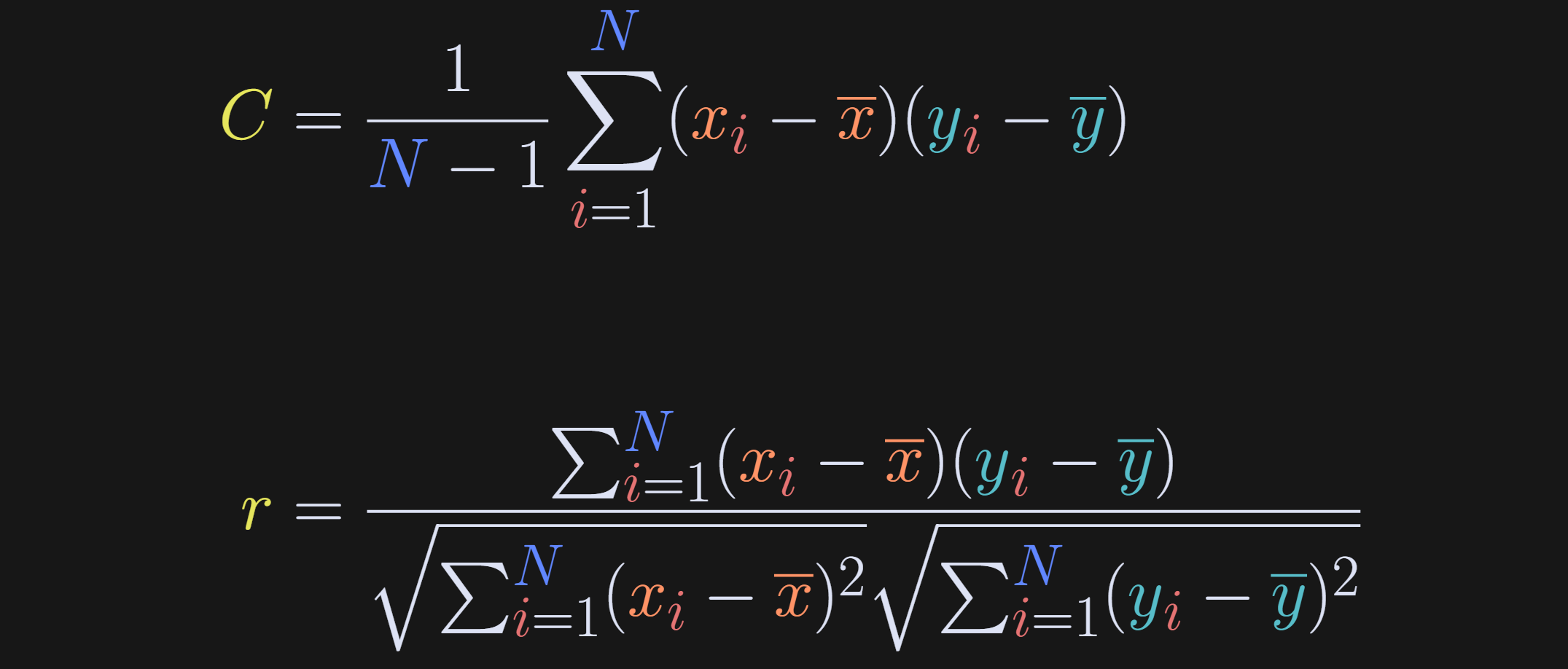
In other words, the correlation coefficient is the covariance in the numerator, and two “auto-covariances” in the denominator.
The 1/(N-1) normalization seems to be missing from the correlation formula. But don’t worry! That scaling factor belongs once in the numerator and twice in the denominator (once under each square root), and thus it cancels from the fraction and is therefore omitted from the equation.
The units cancel in the equation for r: The numerator has units posts-read × happiness, and the denominator has units sqrt(posts-read^2) × sqrt(happiness^2). Side note: units in statistical analyses are often uninterpretable, e.g., what does it mean for “happiness” to be squared or multiplied? Of course we have colloquial interpretations, but those are not mathematically rigorous. Anyway, in practice it’s often best to ignore units and focus on more important things in life — like how to square your happiness instead of square-rooting it ;)
If correlation is easier to interpret and is unit-free, why do we need a measure like covariance? Why not always use correlation?
The answer is that the data scaling actually is important for many analyses, even if the units are difficult to interpret. This is often this case in multivariable analyses, when unique contributions of each variable need to be isolated.
The video below is a detailed walk-through of the code for demo 1.
Demo 2: Covariance to correlation
The goal of this demo is to transform a covariance into a correlation, first by directly translating the equations into code, and then by using the np.corrcoef function to check that the results match.
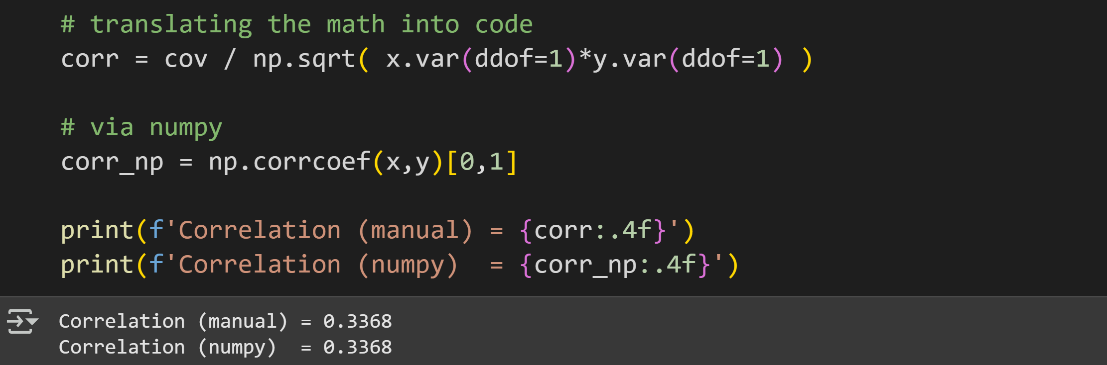
As I wrote in a previous section, translating math directly into code is (imho) one of the best ways to learn data science. But once you feel confident about the implementation, it’s often best to use library-provided functions.
The online code file includes an additional demo that while covariance is sensitive to data scaling, correlation is not.
The main take-home of this subsection is that a correlation coefficient is just a normalized covariance.
Statistical significance of covariance
Covariance does not have a parametric formula for statistical significance, the way that a correlation coefficient does. That is, you cannot determine whether a covariance value is significantly different from zero by plugging in some formula and getting a p-value.
Instead, we can use permutation testing. The idea is to randomly shuffle the data value pairing and recalculate the covariance. “Shuffling” means randomly resorting. Like shuffling a deck of cards to randomize the order.
After hundreds or thousands of shufflings, you’ll get a distribution of permuted covariance values. That’s variously called the null-hypothesis distribution, the H0 (pronounced “h naught” after the British term for “zero”) distribution, or the permuted distribution. Finally, you compare the observed covariance value to the distribution, with the idea being that if the observed value is far outside the H0 distribution, it’s unlikely to be observed by chance, i.e., the observed covariance is statistically significant.
How do you implement the permutation? Segue to the next section…
… but first! A video walk-through of the code for Demo 2:
Demo 3: Statistical significance via permutation testing
There are several ways to shuffle in Python, but all center around the same idea: Randomize the indices. That’s also called permuting or applying a permutation. I think the easiest way to permute indices is using the… wait for it… permutation function :)
Here’s an illustration of how to use numpy’s permutation function.

The output is the indices 0 through 4 (remember that Python is zero-based, so the upper-bound is exclusive), in a random order. Run that code again and you’ll get the same integers in a different order.
Now we just extend that to permuting N indices, and then calculate the covariance between the shuffled x and non-shuffled y.

Why shuffle only x and not y?
The order of the variables doesn’t matter; it’s their pairing that’s important. Imagine the covariance between height and weight in a group of people: It doesn’t matter who we measure in what order — but it does matter that each [height, weight] pair come from the same person. If we swap Bob’s height and Susan’s weight, we wouldn’t expect any meaningful covariance.
Therefore, if we applied the same permuted indices to both variables, then the covariance would be identical. Randomizing the pairing of variables is achieved by permuting only one of the variables.
And how do we interpret that shuffled covariance value of -.55? It is a covariance value we can expect if there is no real relationship between the two variables. In other words, we expect it to be zero, and any deviations from zero can be attributed to noise and random sampling variability.
But that code gives us just one permuted covariance value. The next step is to repeat that procedure many times in a for-loop.

Now we have a distribution of permuted values. The figure below illustrates that distribution with a histogram, and also shows the observed covariance value (without shuffling) as a vertical dashed line.
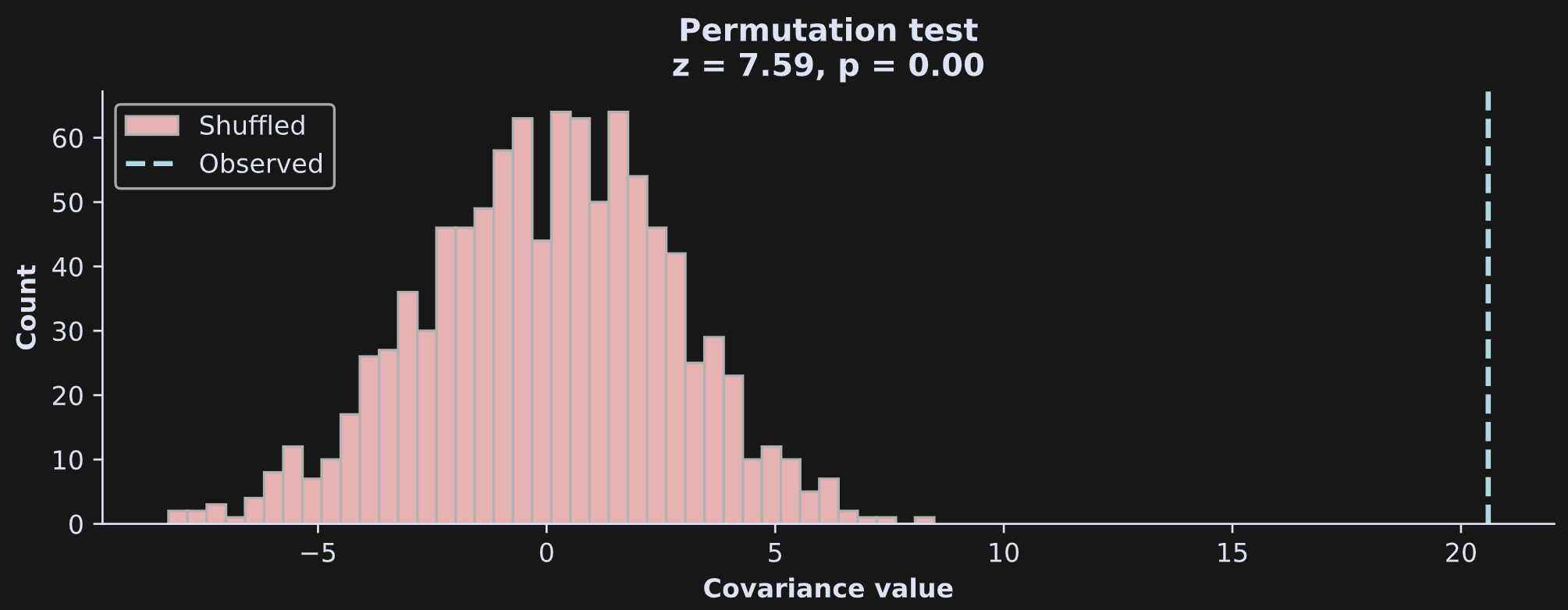
How did I calculate the z and p scores in the title, and what do those values mean?
A z-score is a standardized measure of a data value relative to a distribution. It has units of standard deviations, and, in the context of statistical significance, a large z-score indicates that the observed covariance value is unlikely to occur due to random chance.
The p-value quantifies the probability that the observed value was due to random chance, and is defined as the number of permuted covariance values larger than the observed value. (There are other ways to calculate a permutation p-value, but I’ll use this one for consistency with the next two posts.)
The formulas for z-score and p-value are below.
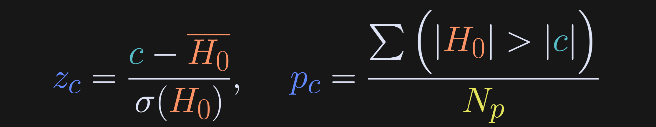
H0 is the null hypothesis distribution, σ() indicates the standard deviation, c is the observed covariance value (the vertical dashed line in the previous figure), and N_p is the number of permutations (1000 in the code demo).
The absolute values in the p-value calculation ensure that the p-value detects significance for both positive and negative covariances. In other words, the p-value reflects how many permuted covariance magnitudes are more extreme than the observed covariance magnitude. You can make it a one-tailed p-value by dropping the absolute value signs (and swapping > to < for a negative covariance).
Here’s the video walk-through for demo 3:
Demo 4: Impact of outliers
Outliers are unusually large values in a dataset. They might come from noise, equipment malfunction, or human data-entry error — or they might be real data values but just unusual. Either way, they can introduce biases into statistical analyses that lead to headaches, misinterpretations, or statistical errors.
There is a lot that can be said about how to identify and deal with outliers, but here I’ll keep the discussion short and more conceptual.
The most common way to identify outliers is by transforming the data to z-scores and then labeling any data value as an outlier if it has an extreme z-score. Those values can then be removed from the data.
But outlier detection for covariance is more nuanced, because we have two variables. There can be outliers in one variable that are not extreme values in the other variable. And to make matters stranger, outliers in different variables can have unpredictable effects on covariance, inflating it, deflating it, or even canceling each other’s deleterious impact.
Consider the code and output below.
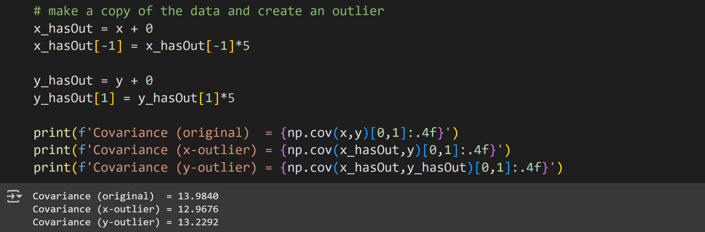
A strange thing happened there: I introduced an outlier by redefining one value to be 5x (using a copy of the data to preserve the original data; that’s good coding!), and that outlier inflated the covariance. But then I introduced another outlier to the other variable, and that actually partly corrected for the first outlier!
Is this a case of two wrongs making a right?
Well, yeah, the second outlier did counteract the deleterious impact of the first outlier to some extent, but that’s not a general phenomenon that you can rely on; it just happened to work out in this case. You can see that in the plot below:
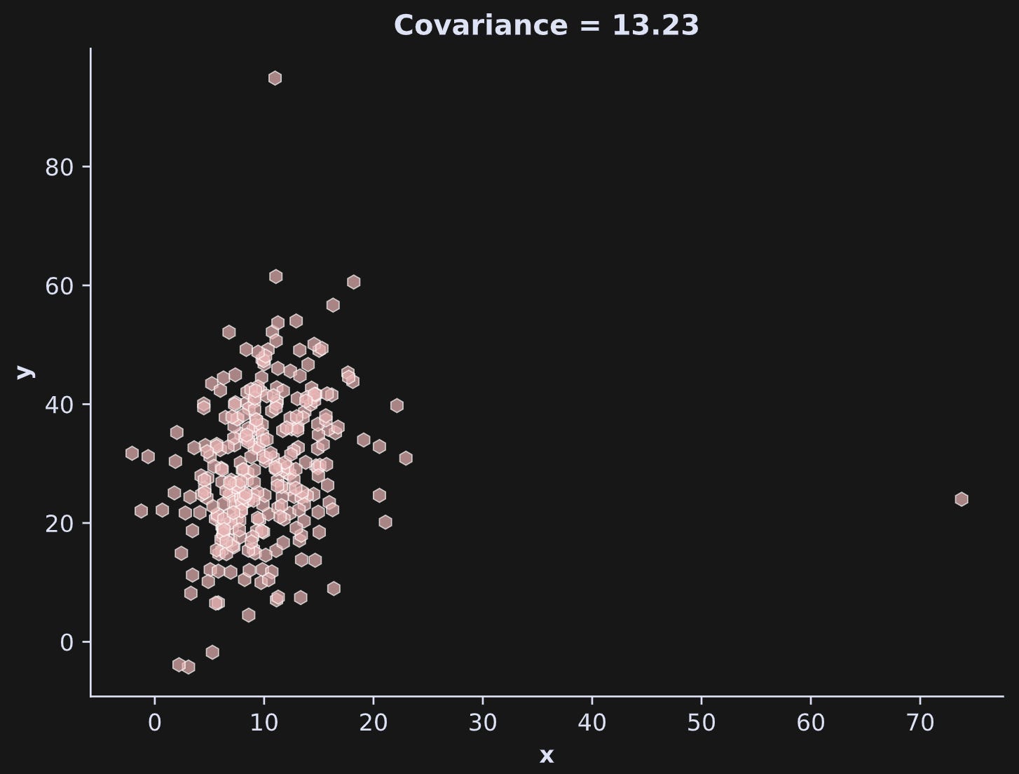
In the interest of preserving my professional integrity, I must admit that I re-ran the code several times to get that “counter-acting” effect; the general phenomenon is that outliers make the covariance unstable; whether the outlier speciously inflates or deflates the covariance depends on the outlier value relative to the distributions of the other variables.
Once you’ve identified outliers, what should you do with them? That’s also a nuanced issue that should be decided on for each dataset and analysis. Some analyses are robust to outliers, but most are negatively impacted by them.
For covariance, outliers are harmful, and removing them is the right thing to do. To identify which outliers should be removed, you can define some z-score threshold, and then remove any data with a z-score greater than that threshold. |z|>4 is a reasonable common threshold — data values four standard deviations away from the mean are uncommon in normally distributed data.
That’s what I show in the figure below.
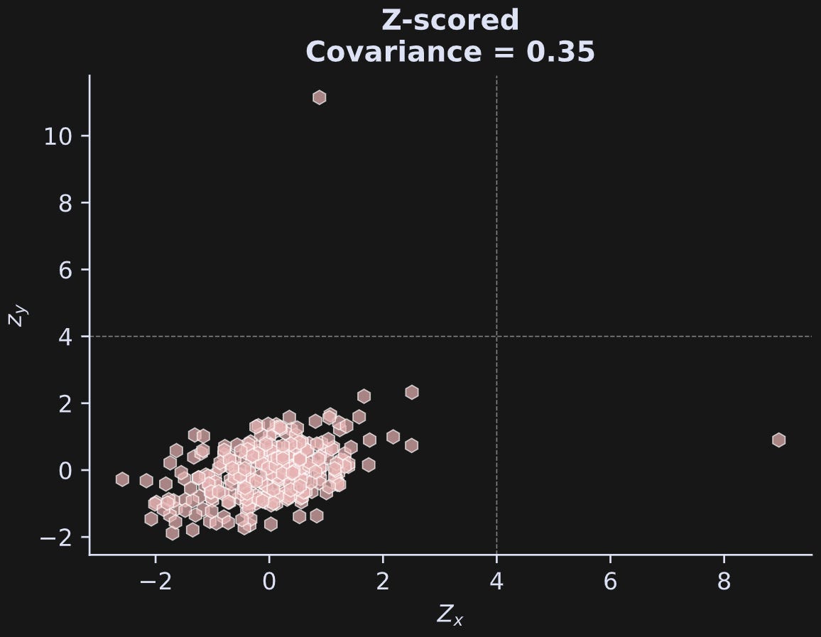
The dashed lines are the thresholds; any data values beyond those thresholds are marked as outliers. These thresholds also apply to negative values, although I didn’t draw those lines in the plot.
Are you surprised that the z-scored covariance is so much smaller than the original-scale covariance? That’s a great example of why covariance values on their own can be difficult to interpret. But do you know what that z-scored covariance is?
It’s the correlation coefficient! The variance of z-scored data is, by definition, 1, which means the correlation formula has only 1’s in the denominator. And the mean is zero. Hence, the covariance of z-scored data is exactly the same as its correlation.
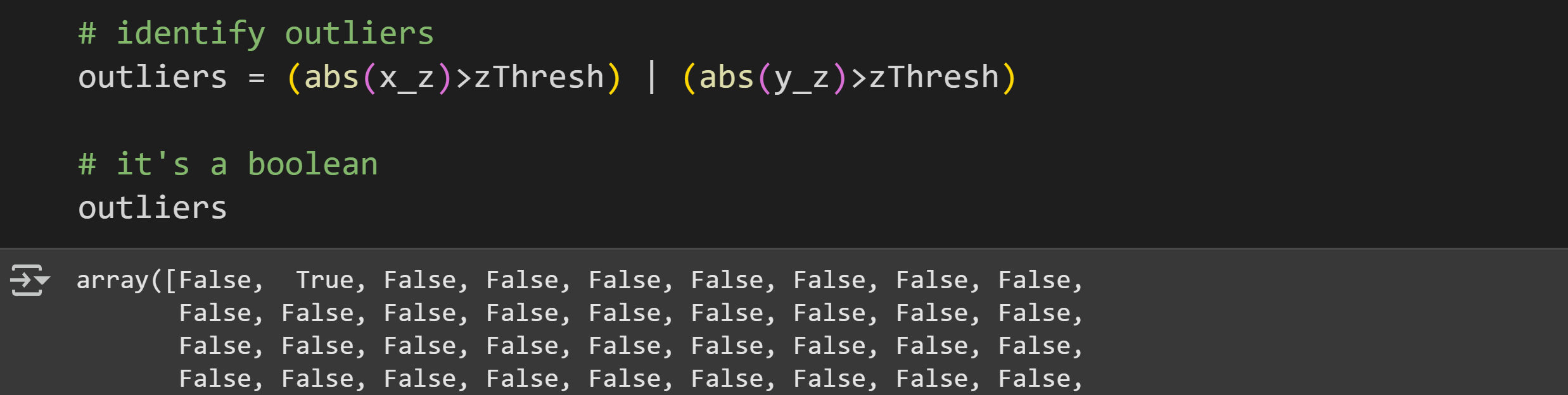
Anyway, now let’s identify those outliers so we can re-calculate covariance without them. The code below shows how I identified pairs of data values in which at least one variable has an outlier.
Now to create a new dataset with the outliers removed:

Notice that the data need to be removed pairwise. That is, when variable x has an outlier, the corresponding value in y needs to be removed, even if that y-value is not extreme.
And here’s the covariance before outliers, with outliers, and with the outliers removed.
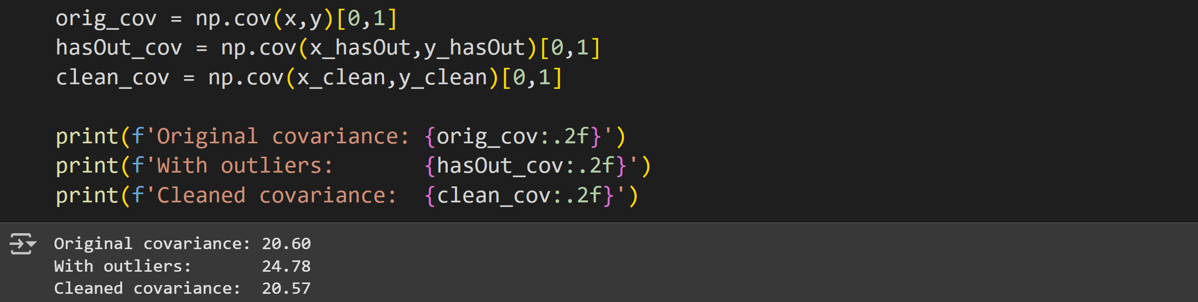
The original and cleaned covariances are not identical, because the cleaned version is missing one data point. However, the cleaned covariance value is a more accurate description of the linear relationship compared to the dataset with the outlier.
One final note about libraries: I wrote this post using numpy. A lot of data science is also done using pandas dataframes. In Post 3 of this series, I’ll use pandas so you can compare the syntax.
And finally, the video for demo 4:
When to use covariance
Covariance may have some disadvantages (the main two being sensitivity to outliers and inability to capture nonlinear interactions), but it really is a workhorse of statistics and machine-learning. Covariances are the basis for correlation, PCA, linear discriminant analysis, optimization, statistical modeling (e.g., least-squares), multivariate signal processing, polynomial regression, solving multivariable differential equations, and many more applications.
Covariances are also are mathematically well-defined and computationally simple and fast. They don’t require sophisticated estimation algorithms or parameters that impact their estimates.
The point is this: don’t confuse linear with limited.
Join me in the next post!
I hope you enjoyed learning about covariance from this post 😁
Post 2 is about mutual information, the cousin of covariance.
What you should do now: Get off your chair, stretch your legs, drink hot coffee and splash cold water on your face (not the other way around); and when you’re ready and refreshed, come back to keep learning!